2.8. Getting Started
2.8.1. R2D Interface
One approach to run the testbed simulation is via the R2D application. After successfully downloading and launching, the major steps for setting up the run are listed as follows:
Set the Units in the GI panel as shown in Fig. 2.8.1.2 and check interested output files.
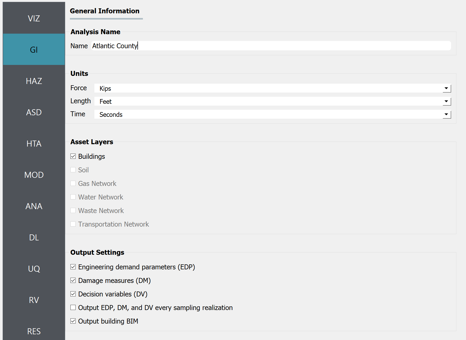
Fig. 2.8.1.2 R2D GI setup.
Download and unzip the HurricaneLaura_MappedPWS. Set the Event File Listing Wind Field in the HAZ panel to the “EventGrid.csv” in the unzipped “IMs” folder. The app would automatically load the directory (Fig. 2.8.1.3). And the Units of Event Input File should be “Miles per hour”.
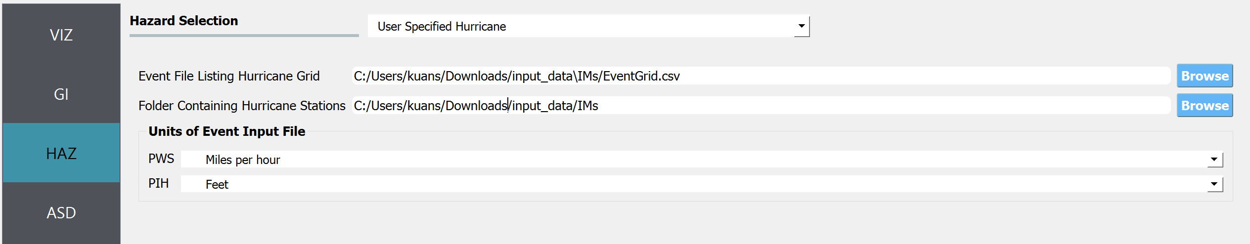
Fig. 2.8.1.3 R2D HAZ setup.
Download the BIM_LakeCharles_Full.csv (under 01. Input: BIM - Building Inventory Data folder). Select CSV to BIM in the ASD panel and set the Import Path to “BIM_LakeCharles_Full.csv” (Fig. 2.8.1.4). Specify the building IDs that you would like to include in the simulation.
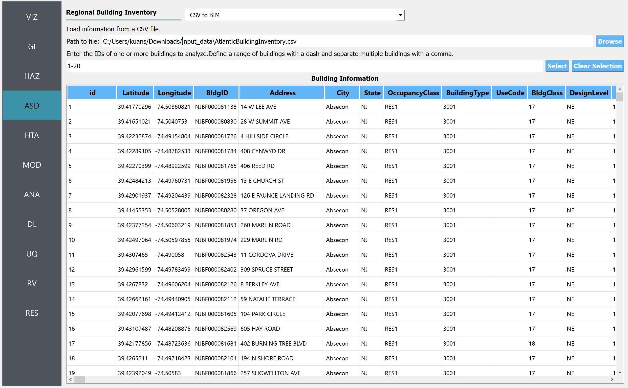
Fig. 2.8.1.4 R2D ASD setup.
Set the Regional Mapping and SimCenterEvent in the HTA panel (e.g., Fig. 2.8.1.5).
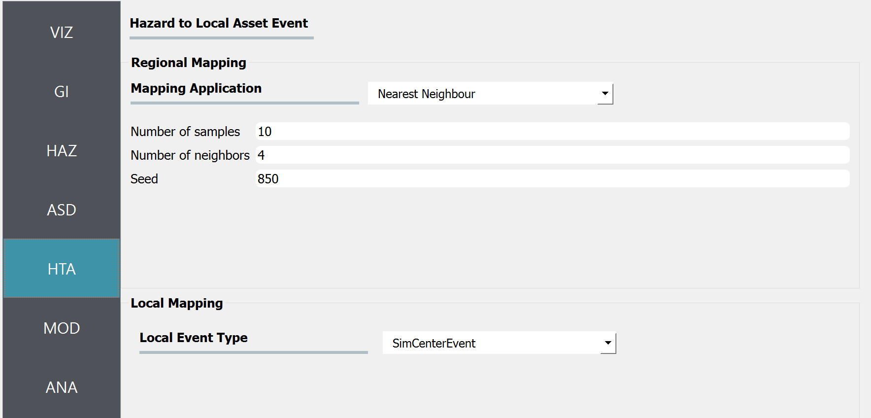
Fig. 2.8.1.5 R2D HTA setup.
Set the “Building Modeling” in MOD panel to “None”.
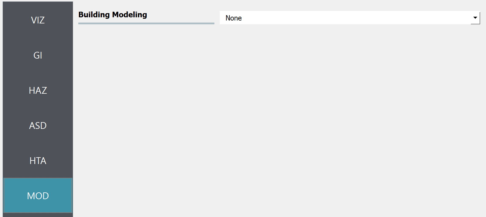
Fig. 2.8.1.6 R2D MOD setup.
Set the “Building Analysis Engine” in ANA panel to “IMasEDP”.
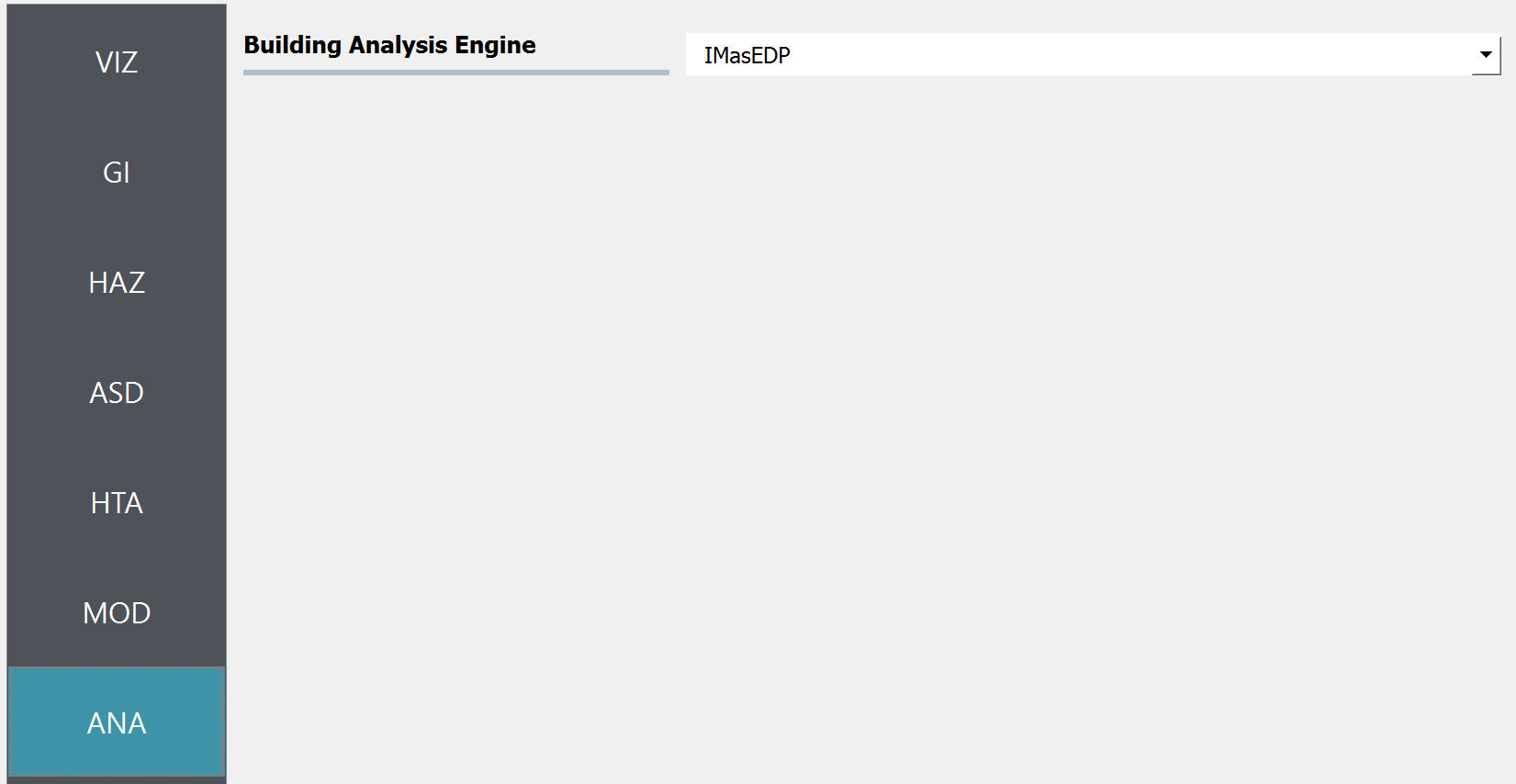
Fig. 2.8.1.7 R2D ANA setup.
Set the “Damage and Loss Method” in DL panel to “HAZUS MH HU”. Download the rulset scripts from DesignSafe PRJ-3207 (under 03. Input: DL - Rulesets for Asset Representation/scripts folder) and set the Auto populate script to “auto_HU_LA.py” (Fig. 2.8.1.8). Note please place the rulset scripts in an individual folder so that the application could copy and load them later.
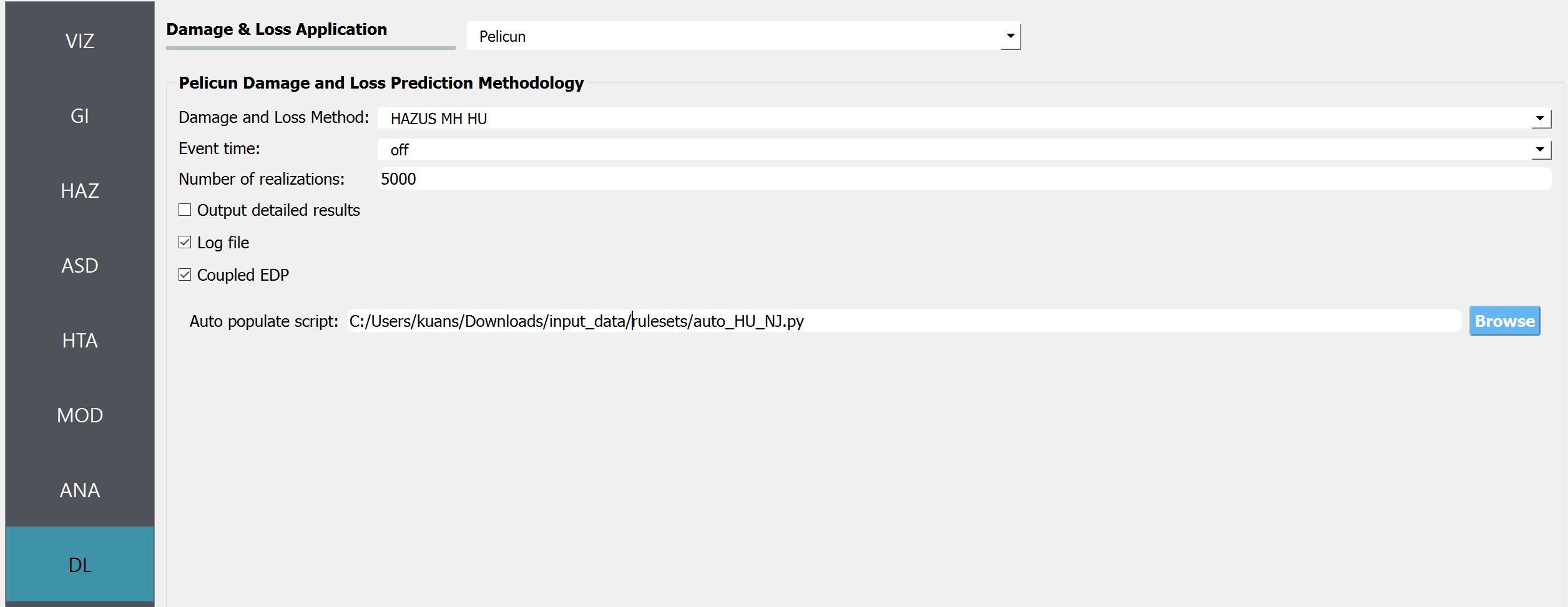
Fig. 2.8.1.8 R2D DL setup.
Set the “UQ Application” in UQ panel to “None”.
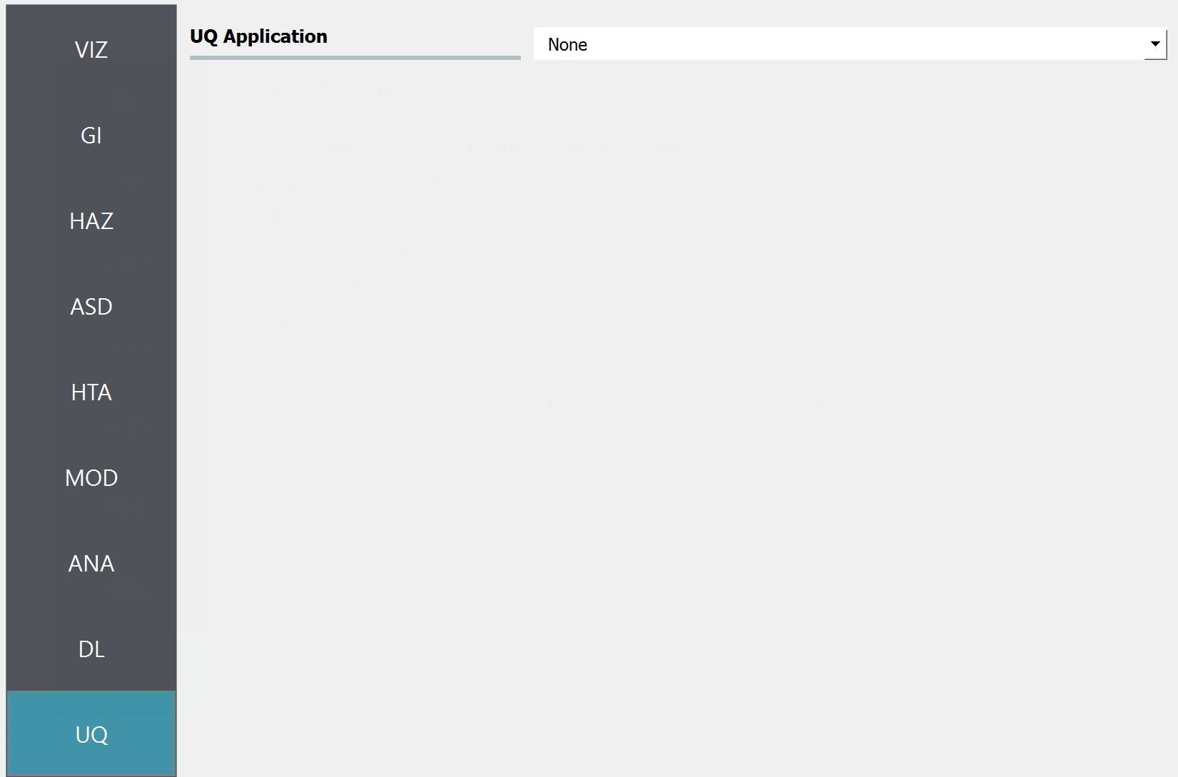
Fig. 2.8.1.9 R2D UQ setup.
After setting up the simulation, please click the RUN to execute the analysis. Once the simulation completed, the app would direct you to the RES panel (Fig. 2.8.1.10) where you could examine and export the results.
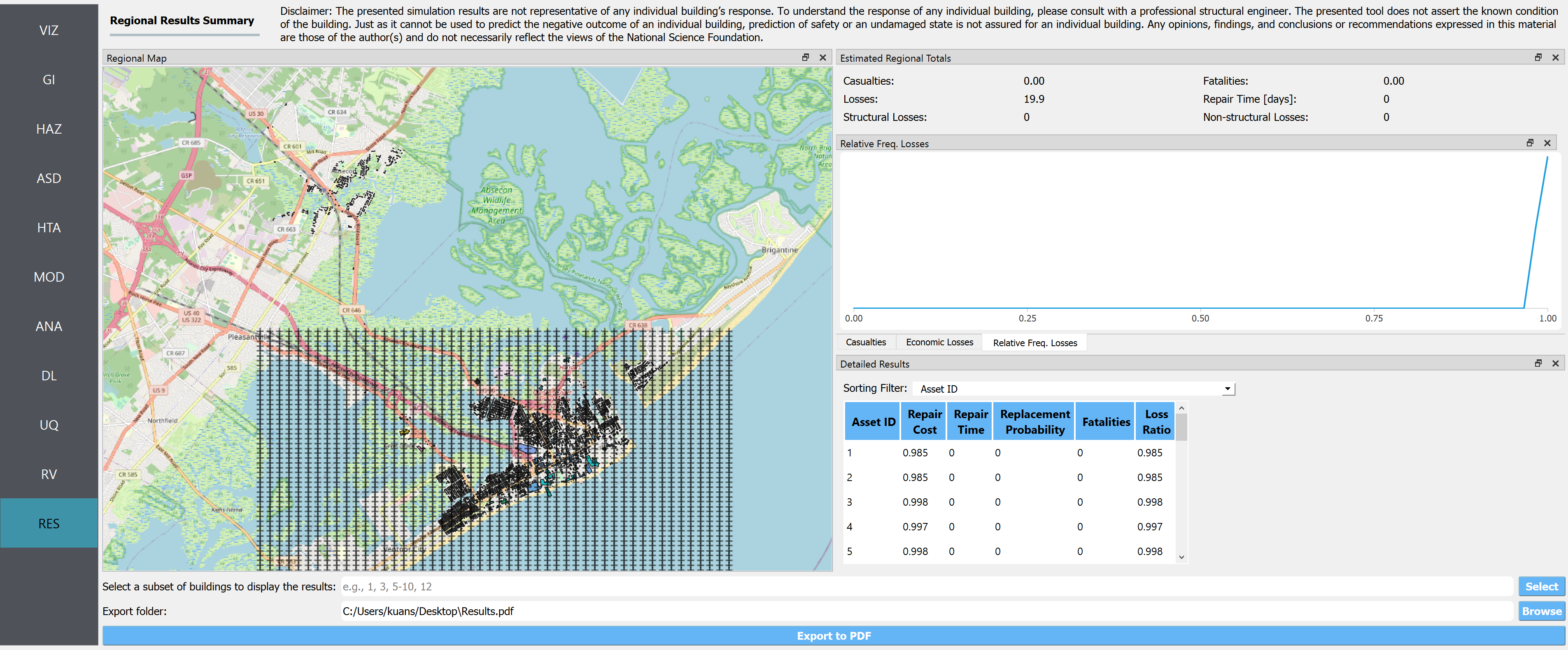
Fig. 2.8.1.10 R2D RES panel.
For simulating the damage and loss for a large region of interest (please remember to reset the building IDs in ASD), it would be efficient to submit and run the job to DesignSafe on Stampede2. This can be done in R2D by clicking RUN at DesignSafe (one would need to have a valid DesignSafe account for login and access the computing resource). Fig. 2.8.1.11 provides an example configuration to run the analysis (and please see R2D User Guide for detailed descriptions). The individual building simulations are paralleled when being conducted on Stampede2 which accelerate the process. It is suggested for the entire building inventory in this testbed to use 20 minutes with 96 Skylake (SKX) cores (e.g., 2 nodes with 48 processors per node) to complete the simulation. One would receive a job failure message if the specified CPU hours are not sufficient to complete the run. Note that the product of node number, processor number per node, and buildings per task should be greater than the total number of buildings in the inventory to be analyzed.
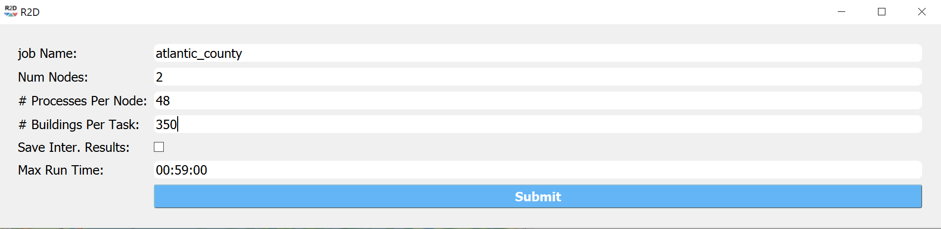
Fig. 2.8.1.11 R2D - Run at DesignSafe (configuration).
Users could monitor the job status and retrieve result data by GET from DesignSafe button (Fig. 2.8.1.12). The retrieved data include four major result files, i.e., BIM.hdf, EDP.hdf, DM.hdf, and DV.hdf. R2D also automatically converts the hdf files to csv files that are easier to work with. While R2D provides basic visualization functionalities (Fig. 2.8.1.10), users could access the data which are downloaded under the remote work directory, e.g., /Documents/R2D/RemoteWorkDir (this directory is machine specific and can be found in File->Preferences->Remote Jobs Directory). Once having these result files, users could extract and process interested information - the next section will use the results from this testbed as an example to discuss more details.
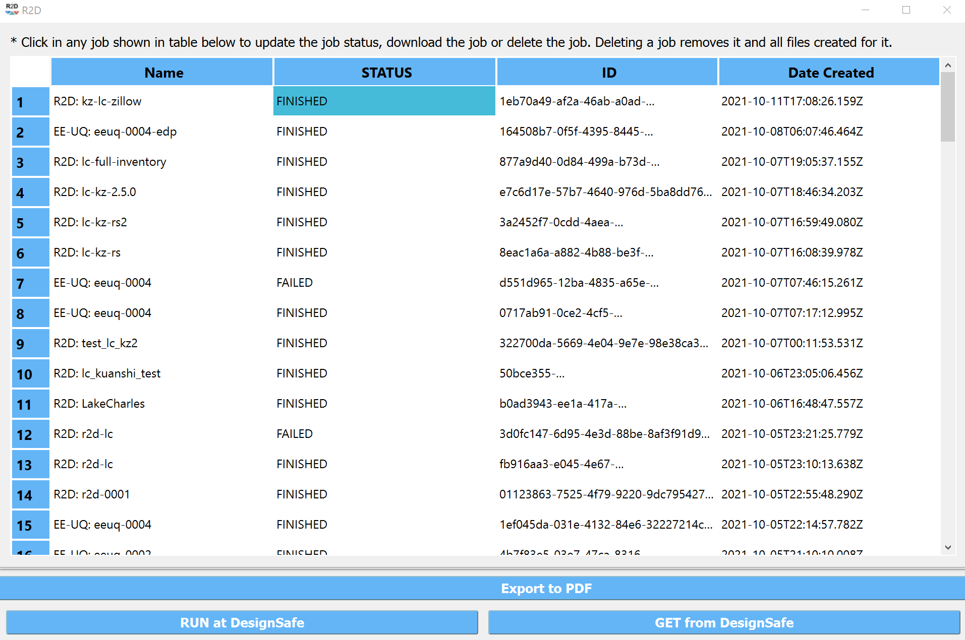
Fig. 2.8.1.12 R2D GET from DesignSafe.
2.8.2. Sample Results
The estimated wind-only, flood-only, and total losses under the four hurricane scenarios (Table 2.3.1.1) are shown in Fig. 2.8.2.1 to Fig. 2.8.2.4.
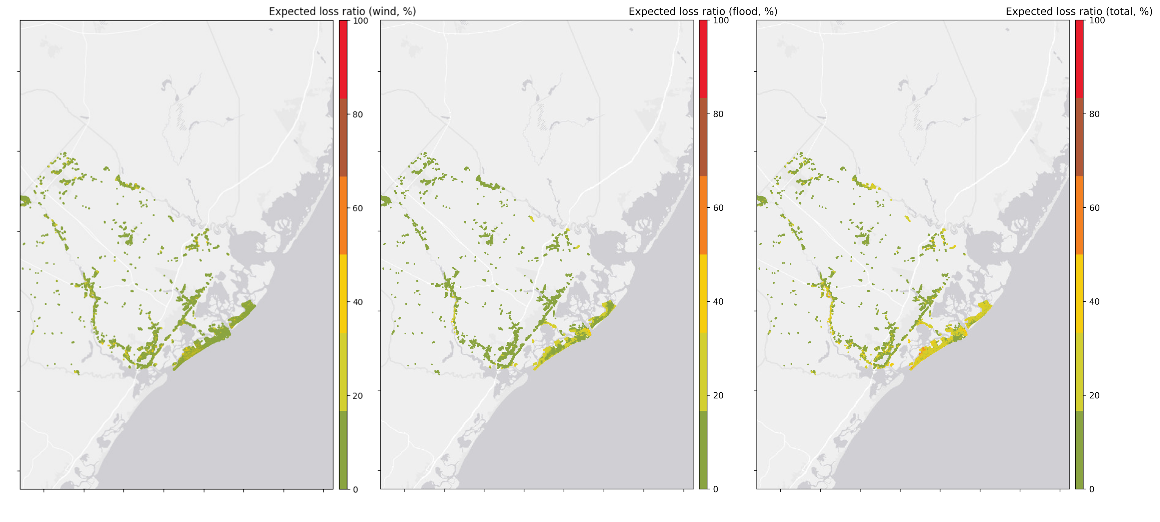
Fig. 2.8.2.1 Estimated regional loss maps for the Category 2 hurricane.
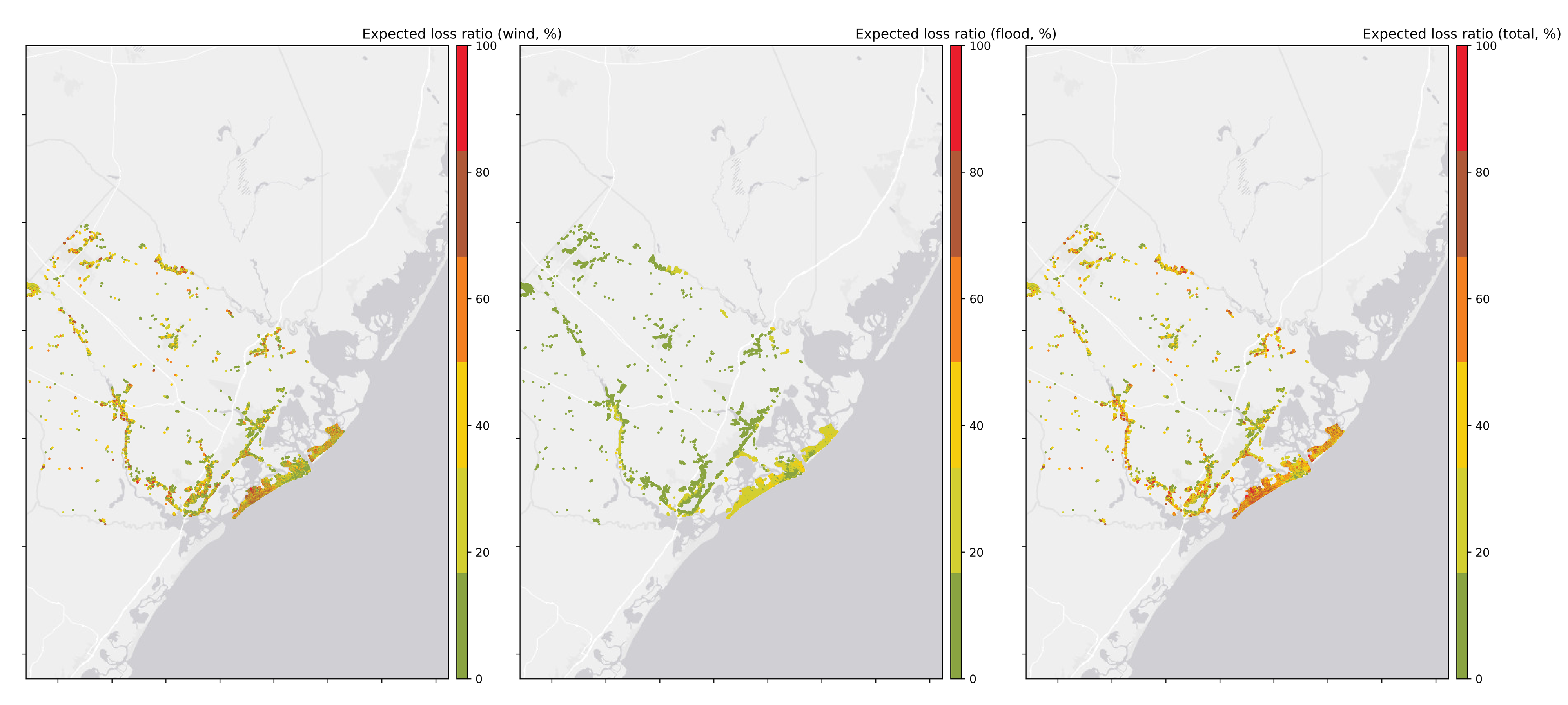
Fig. 2.8.2.2 Estimated regional loss maps for the Category 3 hurricane.
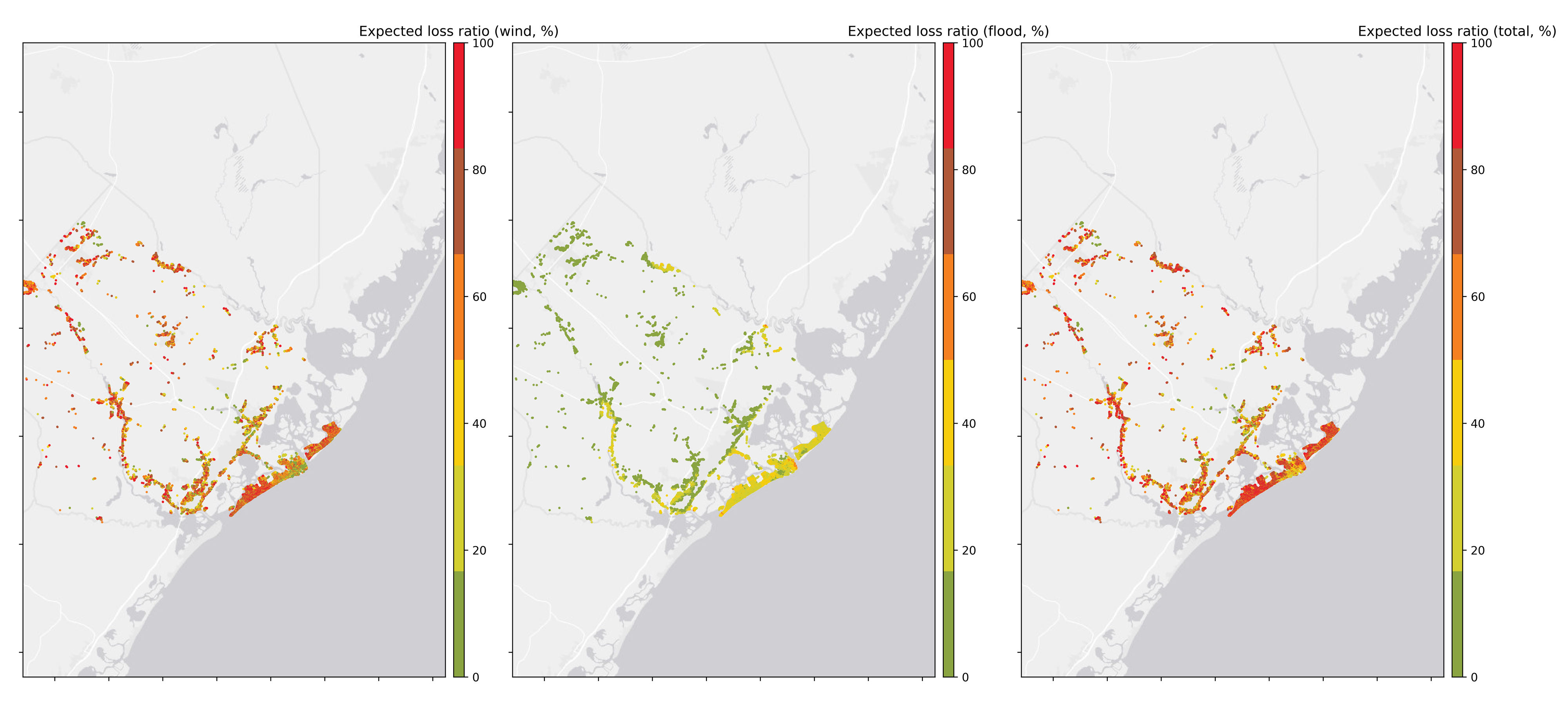
Fig. 2.8.2.3 Estimated regional loss maps for the Category 4 hurricane.
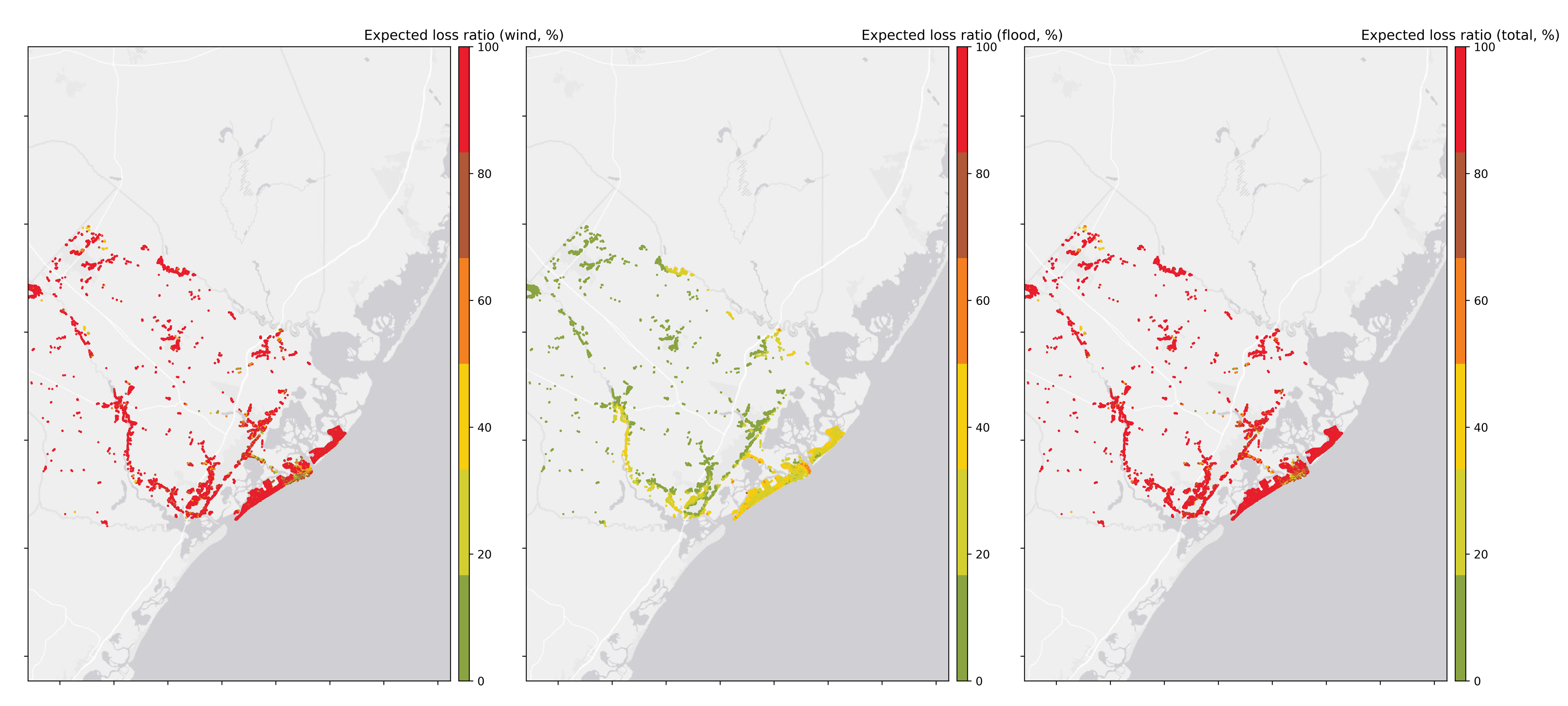
Fig. 2.8.2.4 Estimated regional loss maps for the Category 5 hurricane.
Average expected loss ratios are also computed for individual cities, which are summarized in Fig. 2.8.2.5 to Fig. 2.8.2.8
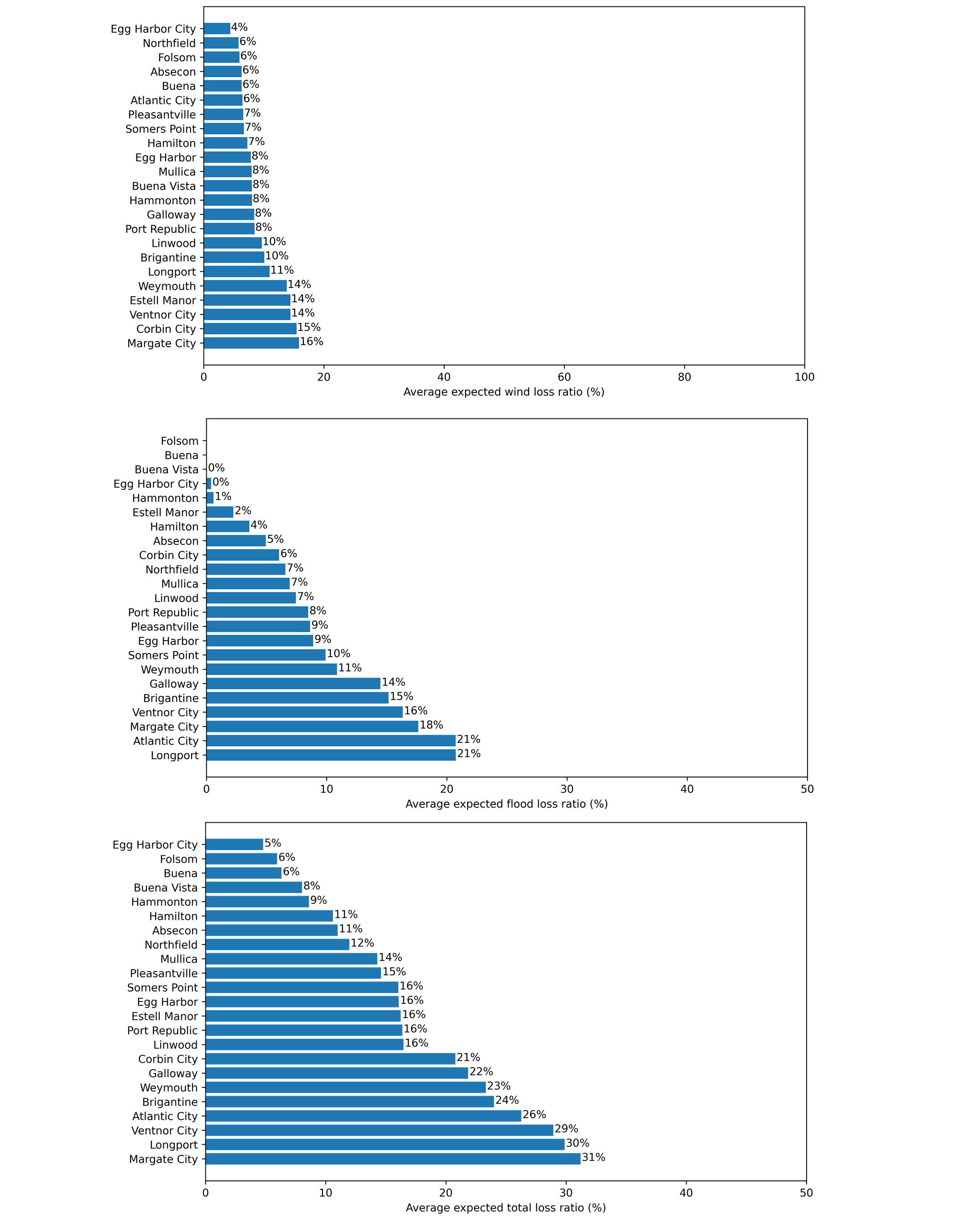
Fig. 2.8.2.5 City-wise average expected loss ratios (Category 2 hurricane).
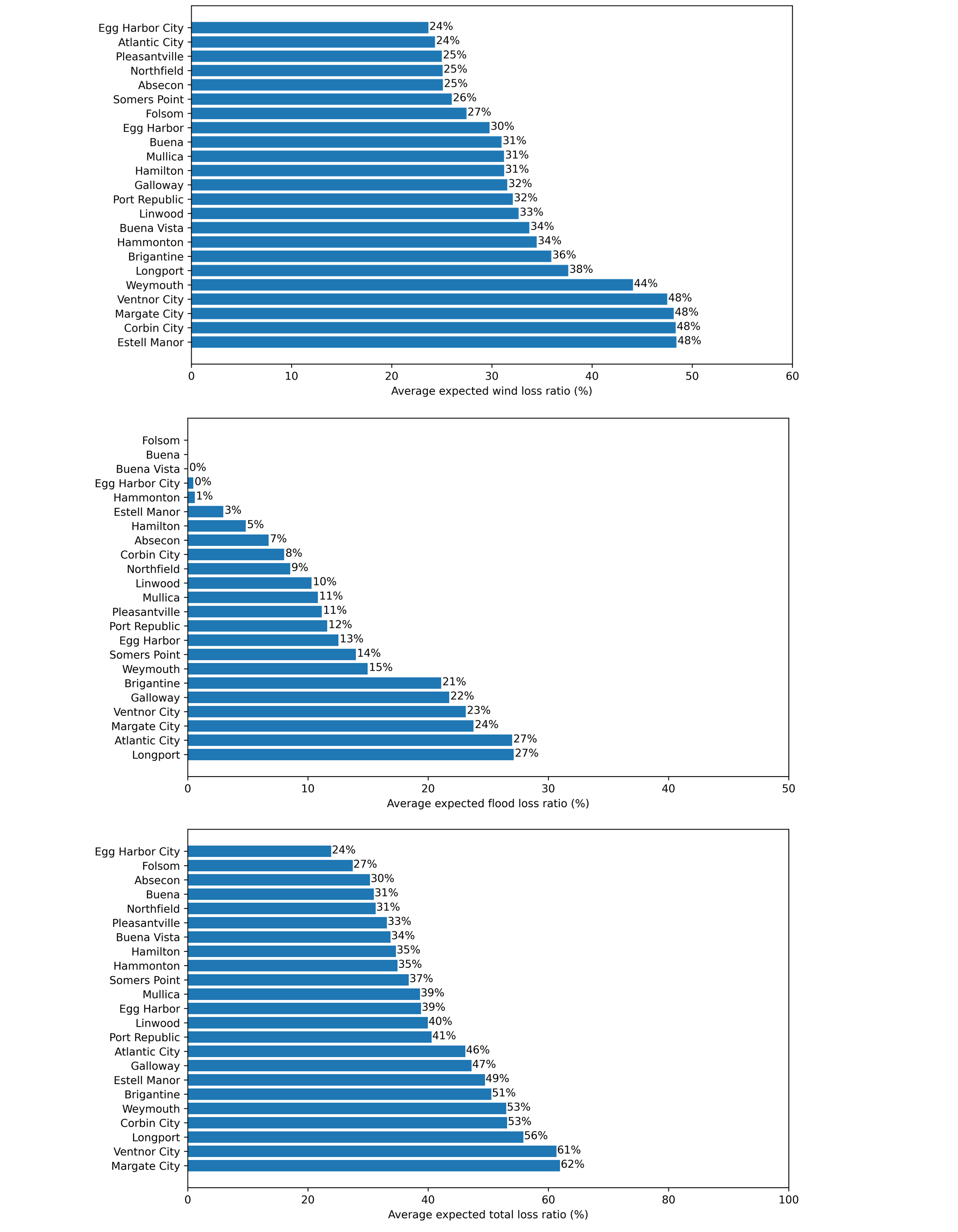
Fig. 2.8.2.6 City-wise average expected loss ratios (Category 3 hurricane).
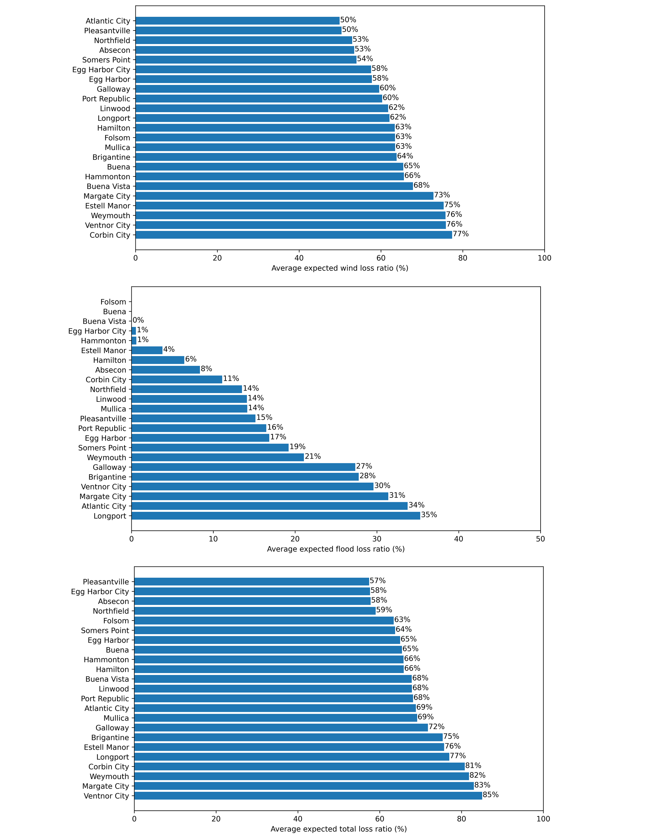
Fig. 2.8.2.7 City-wise average expected loss ratios (Category 4 hurricane).
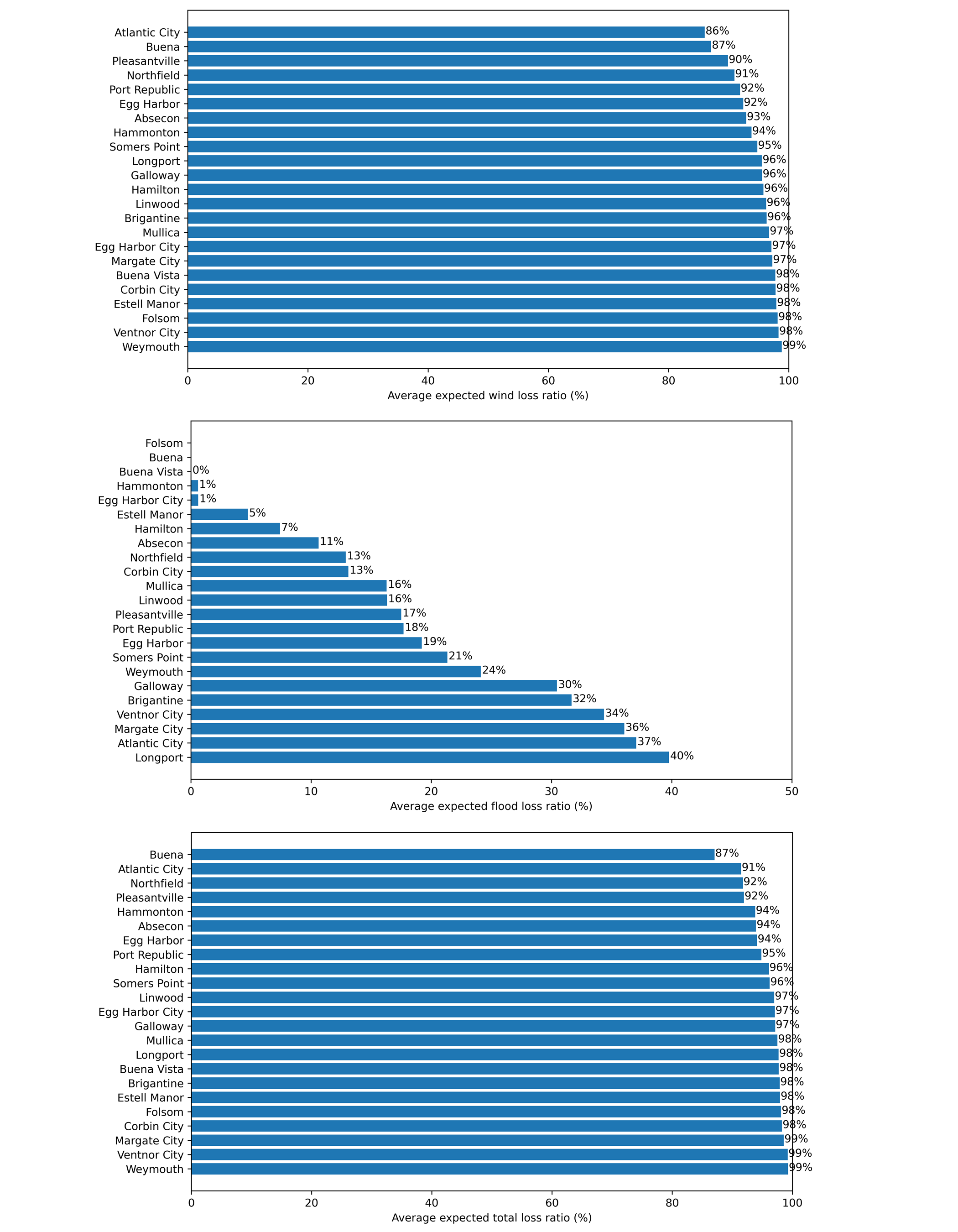
Fig. 2.8.2.8 City-wise average expected loss ratios (Category 5 hurricane).
For the top five cities with most assets in the building inventory, the average expected wind losses are computed for different built eras. Buildings before 1980s generally have relatively higher wind loss ratios where 1970s is found to be the worst decade for Atlantic City, Brigantine, and Galloway. Since 1980, the building performance is improved where the post-2000 buildings are found to behave much better than buildings in the other groups.
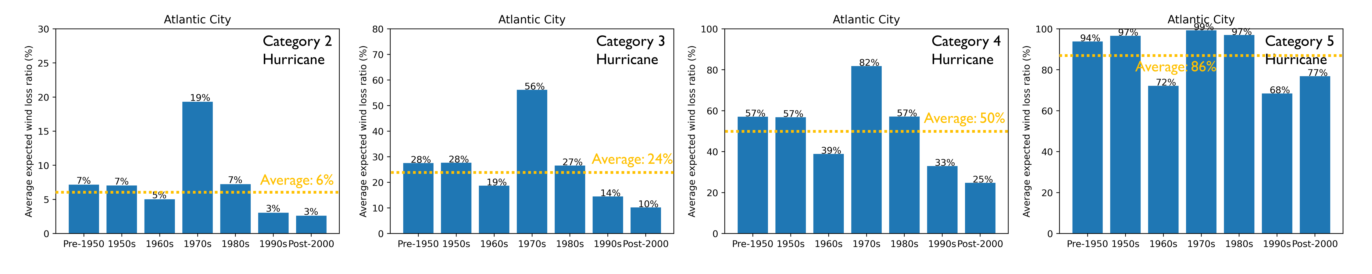
Fig. 2.8.2.9 Average expected wind loss ratios (Atlantic City).
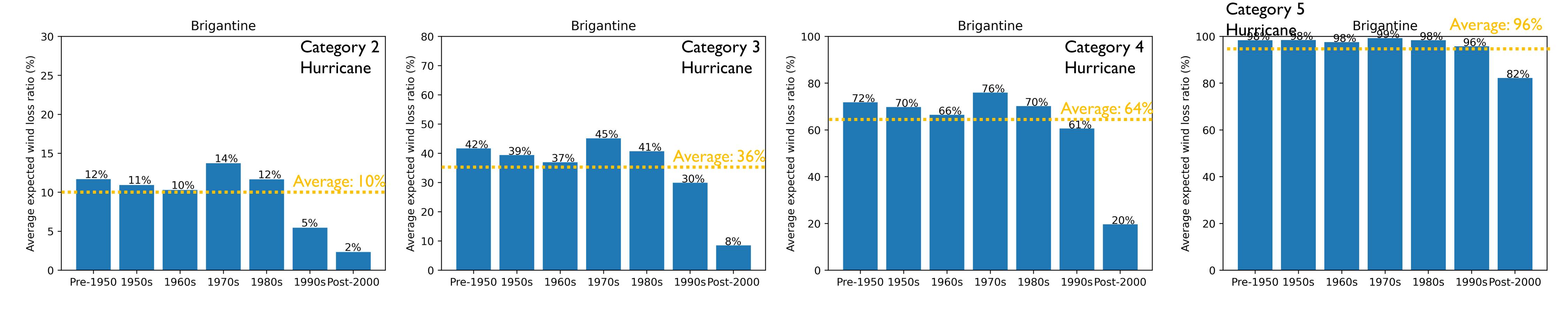
Fig. 2.8.2.10 Average expected wind loss ratios (Brigantine).
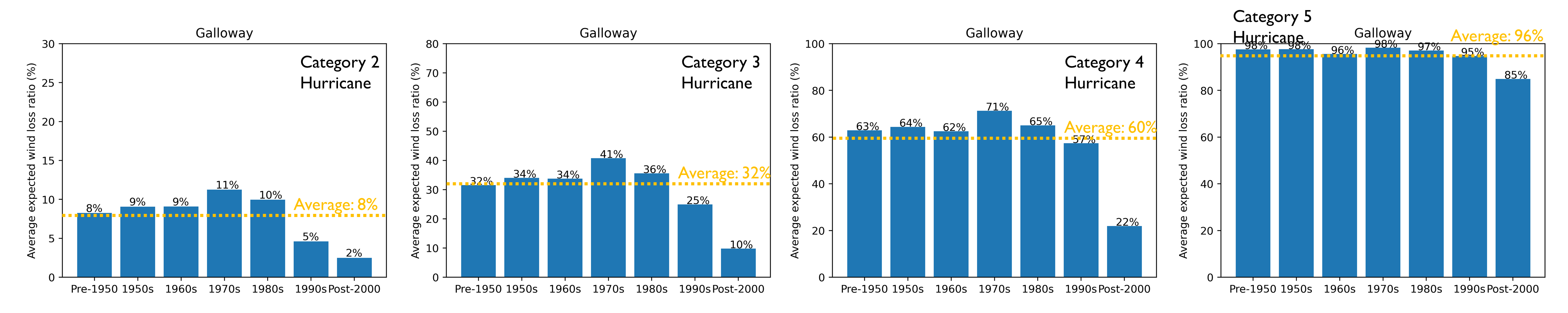
Fig. 2.8.2.11 Average expected wind loss ratios (Galloway).
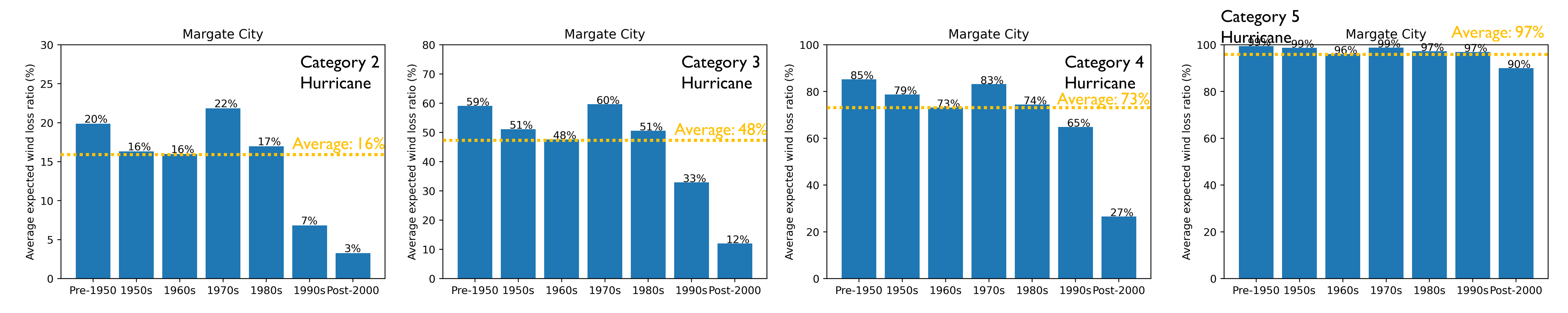
Fig. 2.8.2.12 Average expected wind loss ratios (Margate City).
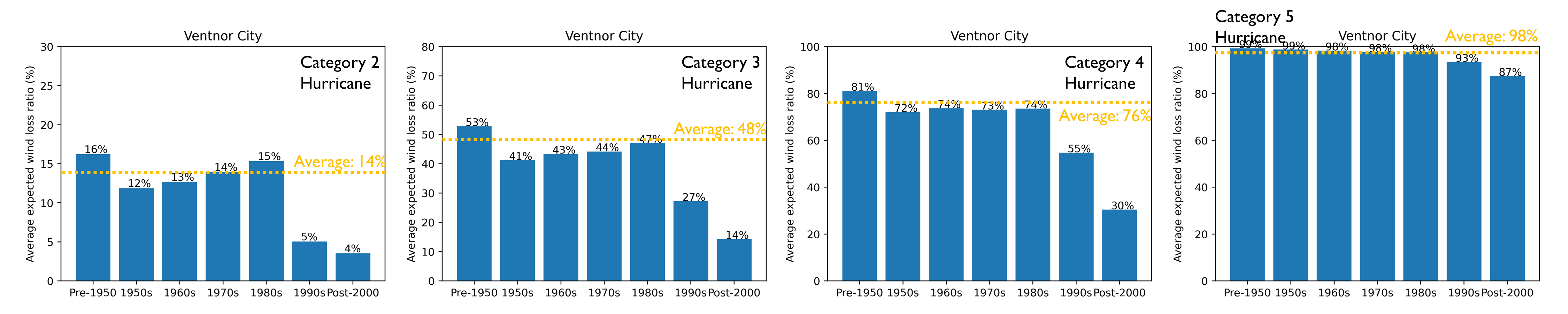
Fig. 2.8.2.13 Average expected wind loss ratios (Ventor City).
The results from the loss estimation for each scenario above (Category 2-5) and each available inventory, can be accessed (Table 2.8.2.1).
Scenario |
Inventory Options |
Location |
|---|---|---|
Scaled Category 2 |
Flood-Exposed Inventory, Exploration Inventory |
|
Scaled Category 3 |
Flood-Exposed Inventory, Exploration Inventory |
|
Scaled Category 4 |
Flood-Exposed Inventory, Exploration Inventory |
|
Category 5 |
Flood-Exposed Inventory, Exploration Inventory |