3.2. Asset Description

This section describes how a large-scale building inventory was constructed in two phases. The initial phase of this work involved identifying the attributes needed. The second phase involved work to obtain these attributes for each building using machine learning and techniques from computer vision to create an initial set of attributes. The remaining attributes were then obtained using other data sources as discussed below.

3.2.1. Phase I: Attribute Definition

All the attributes required for loss estimation were first identified to develop the Building Inventory data model. This Building Inventory data model presented in Table 3.2.1.1 provides a set of attributes that will be assigned to each asset to form the building inventory file serving as input to the workflow. For each attribute a row in the table is provided. Each row has a number of columns: the attribute name, description, format (alphanumeric, floating point number, etc.), the data source used to define that attribute. An expanded version of Table 3.2.1.1 with the full details of this data model are available on DesignSafe PRJ-3207.

Table 3.2.1.1 Building inventory data model, detailed for Lake Charles Inventory.

Description Attribute	Description	Format	Source
ID	Building unique ID.		User defined
Latitude	Latitude of the Building Centroid (inside polygon).	Floating point number (Decimal Degrees)	Microsoft Maps
Longitude	Longitude of the Building Centroid (inside polygon).	Floating point number (Decimal Degrees)	Microsoft Maps
OccupancyClass	Subclassifications of buildings across various categories of Residential (RES), Commercial (COM).	Choices: RES1, RES3, COM1	StreetView
BuildingType	Core construction material type	Choices: Wood	Assume all in wood
YearBuilt	Year of Construction	Integer	StreetView
NumberOfStories	Number of stories estimated via image processing	Integer	StreetView
DWSII	DesignWindSpeed II in mph	Floating point number	ATC API (ASCE 7)
AvgJanTemp	Average temperature in January below or above critial value of 25F.	Choices: Above, Below	User specified
RoofShape	Roof classified into equivalent hip, gable or flat	Choices: Hip, Gable, Flat	Aerial Imagery
RoofSlope	Slope of roof (ratio of rise/vertical over run/horizontal dimensions) covering the majority of the dwelling.	Floating point number	Aerial + StreetView Imagery
MeanRoofHt	Mean height of roof system in ft	Floating point number	Aerial + StreetView Imagery
Garage	Assessor-provided type of garage.	Choices: 0, 1	StreetView
LULC	Land Use Land Cover class	LULC conversion	WebGIS
PlanArea	Plan area (optional)	Floating point number (optional)	User defined or estimated from polygon
AnalysisDefault	Defines the default level of fidelity for analysis	Choices: 1, 2, 3 (optional)	User defined
WindowArea	Window area ratio	Floating point number (optional, default 0.2)	User defined
WindZone	Rating of the amount of wind pressure a manufactured home	Choice: I, II, III, IV (optional, default I)	User defined
RoofSystem	Roof system	Choices: Wood, OWSJ (optional, default Wood)	User defined
SheathingThickness	Thickness of sheathing (inch)	Floating point number (optional, default 1.0)	User defined
FloodZone	FEMA FloodZone designation as defined by Flood Insurance Rate Maps	FEMA designation (optional, default X)	User specified
Representation Attribute	Description	Format	Source
HazusClassW	Hazus building classes as defined for wind hazards	Choices: WSF1-2, WMUH1-3	Rulesets (see Asset Representation)
HazardProneRegion	Hazard Prone Regions for Hazus wind vulnerability assignments for WSF1-2	Choices: yes, no	Rulesets (see Asset Representation)
WindBorneDebris	Wind Borne Debris for Hazus wind vulnerability assignments for WSF1-2	Choices: yes, no	Rulesets (see Asset Representation)
SecondaryWaterResistance	Secondary Water Resistance for Hazus wind vulnerability assignments for WSF1-2, WMUH1-3	Choices: yes, no	Rulesets (see Asset Representation)
RoofCover	Roof cover for Hazus wind vulnerability assignments for WMUH1-3	Choices: N/A, BUR, SPM	Rulesets (see Asset Representation)
RoofQuality	Roof cover quality for Hazus wind vulnerability assignments for WMUH1-3	Choices: N/A, poor, good	Rulesets (see Asset Representation)
RoofDeckAttachmentW	Roof Deck Attachment for wood for Hazus wind vulnerability assignments for WSF1-2, WMUH1-3	Choices: A, B, C, D	Rulesets (see Asset Representation)
RoofToWallConnection	Roof to Wall Connection for Hazus wind vulnerability assignments for WSF1-2, WMUH1-3	Choices: strap, toe-nail	Rulesets (see Asset Representation)
Shutters	Window opening protection for Hazus wind vulnerability assignments for WSF1-2, WMUH1-3, MMUH1-3	Choices: yes, no	Rulesets (see Asset Representation)
AugmentedGarage	Attached garage for Hazus wind vulnerability assignments for WSF1-2	Choices: none, SFBC 1994, standard, weak	Rulesets (see Asset Representation)
TerrainRoughness	HAZUS-defined terrain classification (x100) based on LULC data	Choices: 3, 15, 35, 70, 100	Rulesets (see Asset Representation)

3.2.2. Phase II: Inventory Generation

This section describes how the large-scale building inventory was constructed for Lake Charles using a phased approach that used machine learning, computer vision algorithm and data distributions to generate all attributes required for the corresponding loss assessment. It is emphasized that the intent is to demonstrate how an inventory could be constructed and not to address potential errors, omissions or inaccuracies in the source data, i.e., source data are assumed to be accurate and no additional quality assurance was conducted outside of addressing glaring omissions or errors.

For each of the attributes identified in Table 3.2.1.1, a description of the attribute and information on how the data was identified and validated is presented.

AI/ML Techniques combined with Computer Vision

Many of those attributes were generated with the SimCenter’s BRAILS CityBuilder application. To avoid replication in the text, the following describes how those attributes were obtained. The sections below will present the validation of the data.

CityBuilder is a python application that incorporates different AI/ML modules from BRAILS for performing specific tasks. The user creates a python script importing City Builder, constructing a CityBuilder object and then asking that object to build the inventory. The example script shown below, albeit our GoogleMapAPIKey removed, will create a building inventory file for use in the workflow.

# Import the module from BRAILS
from brails.CityBuilder import CityBuilder
# Initialize the CityBuilder
cityBuilder = CityBuilder(attributes=['occupancy','roofshape'],
                  numBldg=10,random=True, place='Lake Charles, Louisiana',
                  GoogleMapAPIKey='REMOVED GOOGLE API KEY')
# create the city-scale BIM file
BIM = cityBuilder.build()

Upon execution, CityBuilder will:

1. Download footprints for all buildings in the interested region, Lake Charles, from the Microsoft Footprint Dataset ([Microsoft18]).

2. Calculates the coordinate (Latitude, Longitude) for each building’s centroid, based on the footprint information.

3. Download both a satellite image and a street view image for each building using Google API’s and the extracted coordinates.

4. Perform computations on the images to obtain the interested building attributes using a series of pre-trained AI models.

Attribute: RoofShape

The RoofShape is obtained by CityBuilder using the BRAILS Roof shape module. The roof shape module determines roof shape based on a satellite image obtained for the building. The module uses machine learning, specifically it utilizes a convolutional neural network that has been trained on satellite images. In AI/ML terminology the Roof Shape module is an image classifier: it takes an image and classifies it into one of three categories used in HAZUS: gable, hip, or flat as shown in Fig. 3.2.2.1. The original training of the AI model utilized 6,000 images obtained from google satellite imagery in conjunction with roof labels obtained from Open Street Maps. As many roofs have more complex shapes, a similitude measure is used to determine which of these roof geometries is the best match to a given roof. More details of the classifier can be found here. The trained classifier was employed here to classify the roof information for Lake Charles.

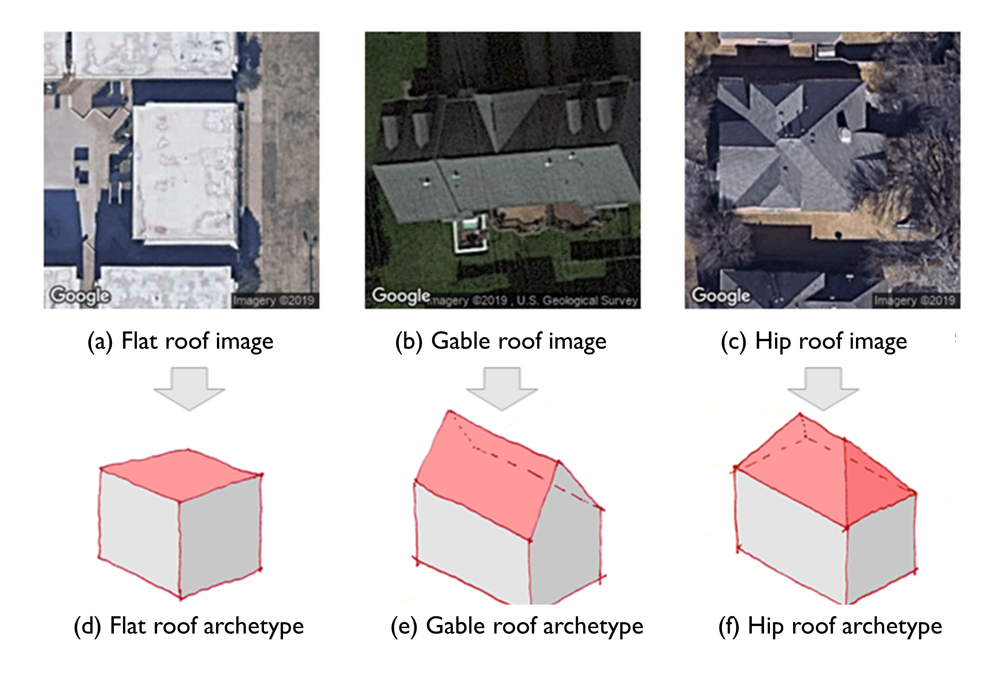
Fig. 3.2.2.1 Roof type classification with examples of aerial images (a-f) and simplified archetypes (d-f) used by Hazus.

The performance of the roof shape classifier was validated against two ground truth datasets. The first is comprised of 125 manually labeled satellite images sampled from OpenStreetMap from across the US, retaining only those with unobstructed views of building roofs (a cleaned dataset). The second is 56 residences assessed by StEER for which roof types were one of the three HAZUS classes, e.g., removing all roofs labeled as “Complex” according to StEER’s distinct image labeling standards. The validation process is documented here. The confusion matrices are presented in Fig. 2.2.2.7. These matrices visually present the comparison between the predictions and actual data and should have values of 1.0 along the diagonal if the classification is perfect, affirming the accuracy of the classification by the roof shape classifier.

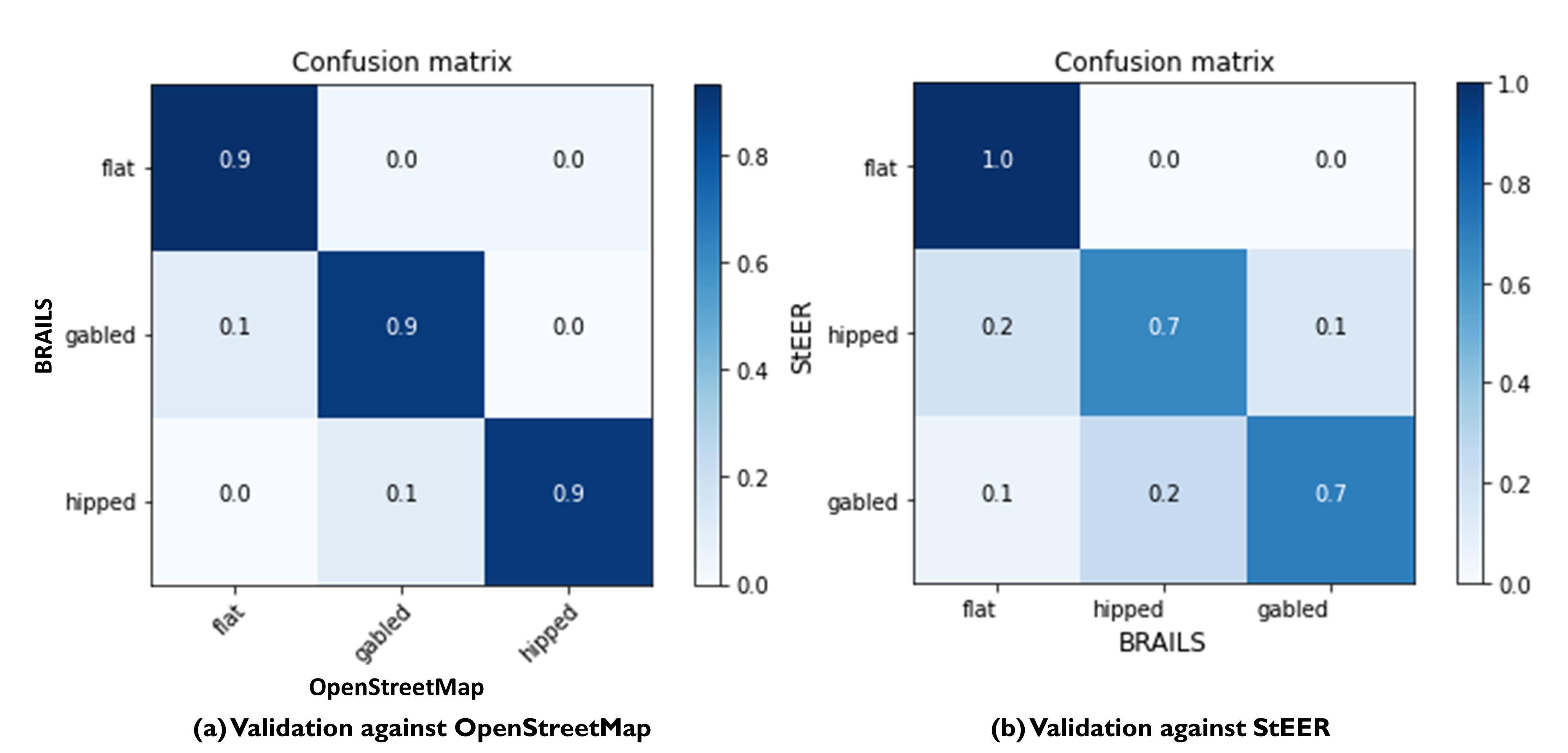
Fig. 3.2.2.2 Validation of BRAILS predicted roof shapes to roof shapes from OpenStreetMap and StEER.

Attribute: OccupancyClass

The occupancy class attribute is also determined by CityBuilder using the occupancy class classifier module in BRAILS. The occupancy classifier is also a convolutional neural network. This network trained using 15,743 google street view images with labels derived from OpenStreetMaps and the NJDEP dataset in the Atlantic County, NJ testbed Asset Description. This classifier labels buildings as one of: RES1 (single family building), RES3 (multi-family building), COM1 (Commercial building). More details of the classifier can be found here.

The performance of the classifier was validated against a ground truth dataset that contains 293 street view images from the United States with unobstructed views of the buildings (cleaned data). The full validation was documented here. The confusion matrix, which presents visually the predictions versus actual data from the original 293 image validation set, is as shown in Fig. 3.2.2.3 for OpenStreetMaps (see plot a), and the NJDEP dataset (see plot b). Fig. 3.2.2.4 displays the BRAILS occupancy predictions for Lake Charles for a selected region. Note that only those classified as RES1 or RES3 are retained in this testbed focused on residential construction (and the COM1 is assigned to the buildings that are classified other than the two residential classes by BRAILS).

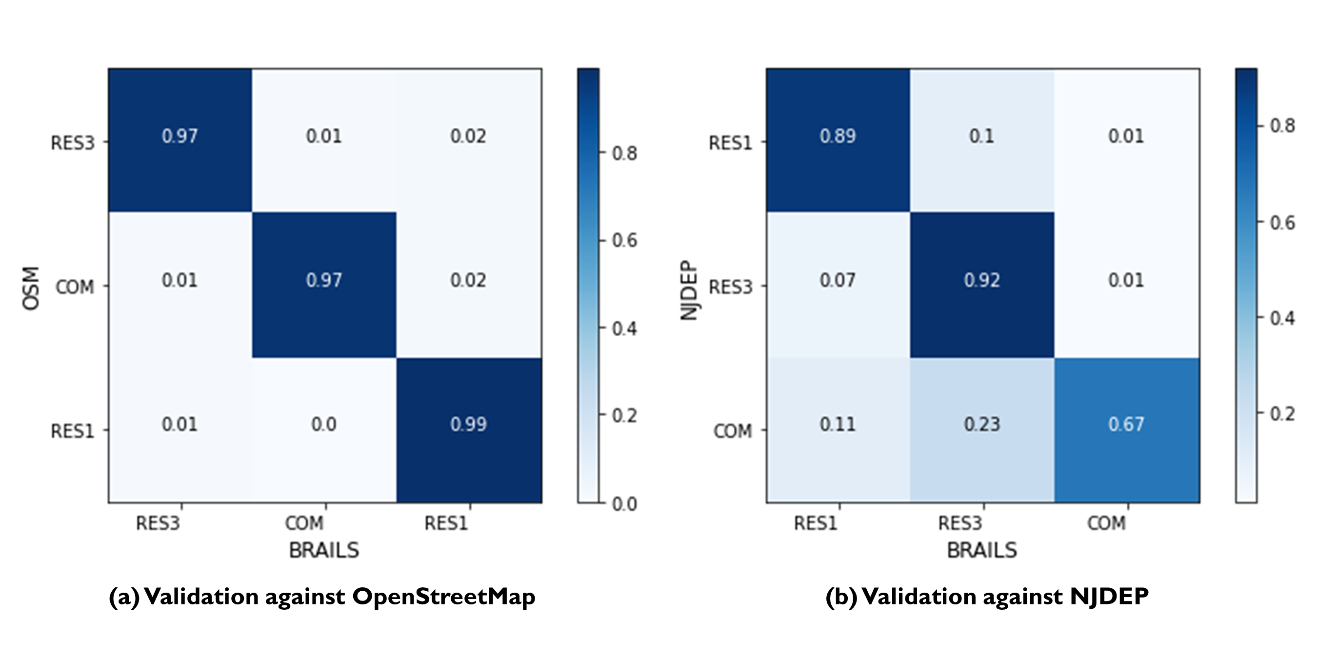
Fig. 3.2.2.3 Validation of BRAILS predicted occupancy classes to OpenStreetMap and NJDEP.

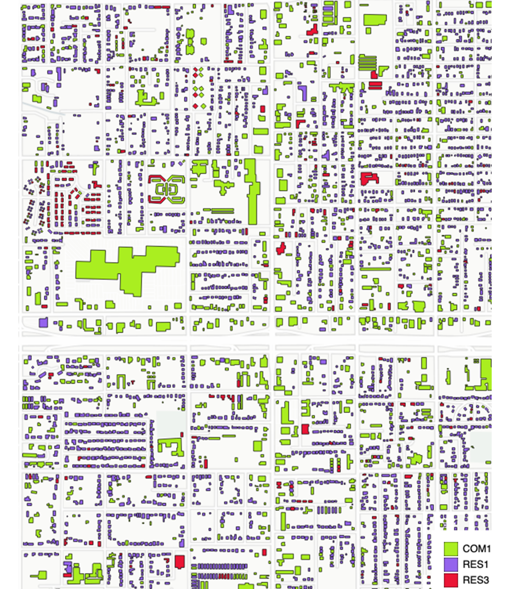
Fig. 3.2.2.4 AI predicted occupancy types from street view images in Lake Charles.

Attribute: NumberOfStories

This attribute is determined by CityBuilder using an object detection procedure. A detection model that can automatically detect rows of building windows was established to generate the image-based detections of visible floor locations from street-level images. The model was trained on the EfficientDet-D7 architecture with a dataset of 60,000 images, using 80% for training, 15% for validation, and 5% testing of the model. In order to ensure faster model convergence, initial weights of the model were set to model weights of the (pretrained) object detection model that, at the time, achieved state-of-the-art performance on the 2017 COCO Detection set. For this specific implementation, the peak model performance was achieved using the Adam optimizer at a learning rate of 0.0001 (batch size: 2), after 50 epochs. Fig. 3.2.2.5 shows examples of the floor detections performed by the model.

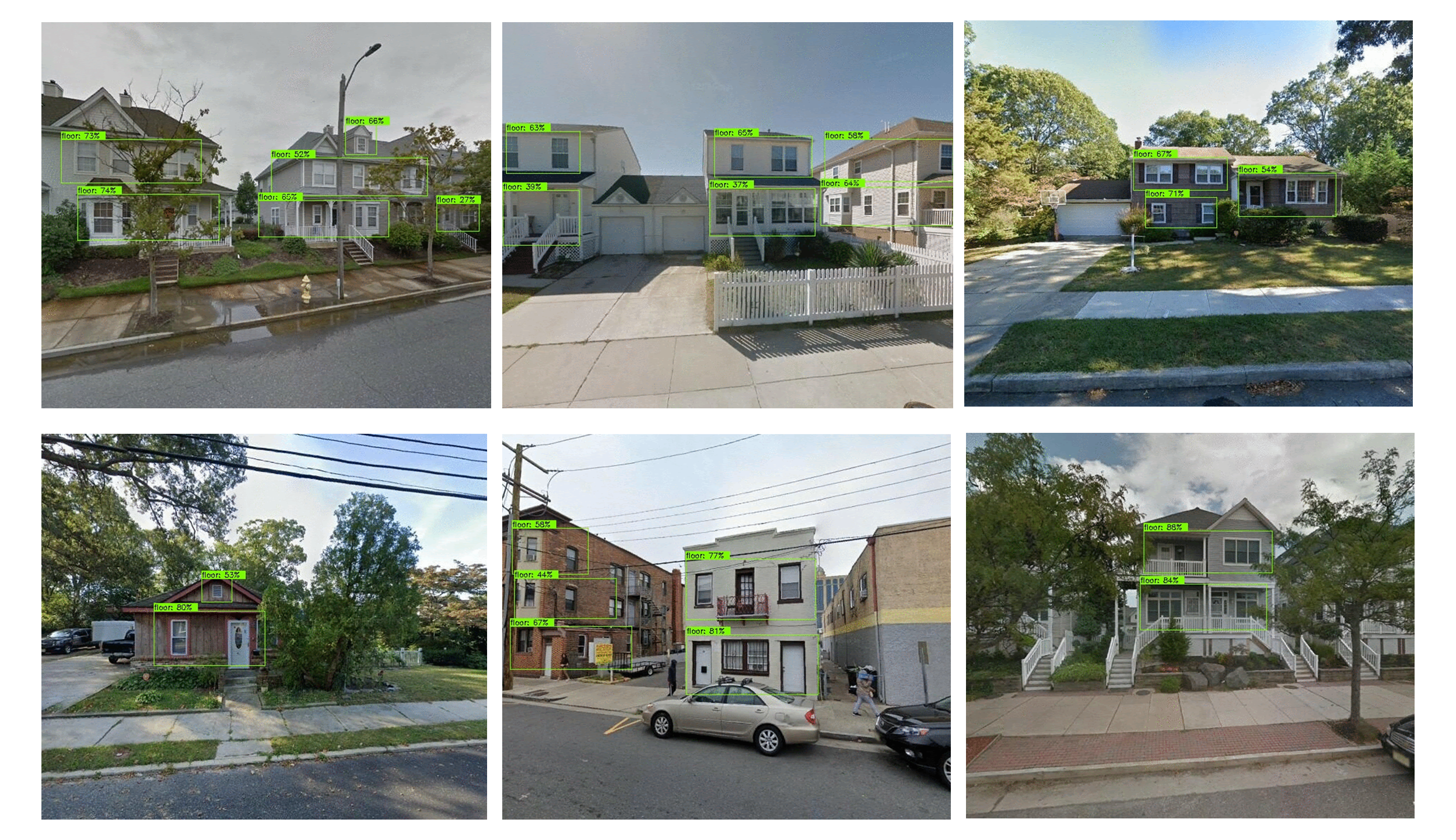
Fig. 3.2.2.5 Sample floor detections of the floor detection model (each detection is indicated by a green bounding box). The percentage value shown on the top right corner of a bounding box indicates model confidence level associated with that prediction.

For an image, the described floor detection model generates the bounding box output for its detections and calculates the confidence level associated with each detection (see Fig. 3.2.2.5). A post-processor that converts stacks of neighboring bounding boxes into floor counts was developed to convert this output into floor counts. Recognizing an image may contain multiple buildings at a time, this post-processor was designed to perform counts at the individual building level.

For a random image dataset of buildings captured using arbitrary camera orientations (also termed in the wild images), the developed floor detection model was determined to capture the number of floors information of buildings with an accuracy of 86%. Fig. 2.2.2.2 (a) provides a breakdown of this accuracy measure for different prediction classes (i.e. the confusion matrix of model classifications). It was also observed that if the image dataset is established such that building images are captured with minimal obstructions, the building is at the center of the image, and perspective distortions are limited, the number of floors detections were performed at an accuracy level of 94.7% by the model. Fig. 2.2.2.2 (b) shows the confusion matrix for the model predicting on the “cleaned” image data. In quantifying both accuracy levels, a test set of 3,000 images randomly selected across all counties of a companion testbed in New Jersey, excluding Atlantic County (site of that testbed), was utilized.

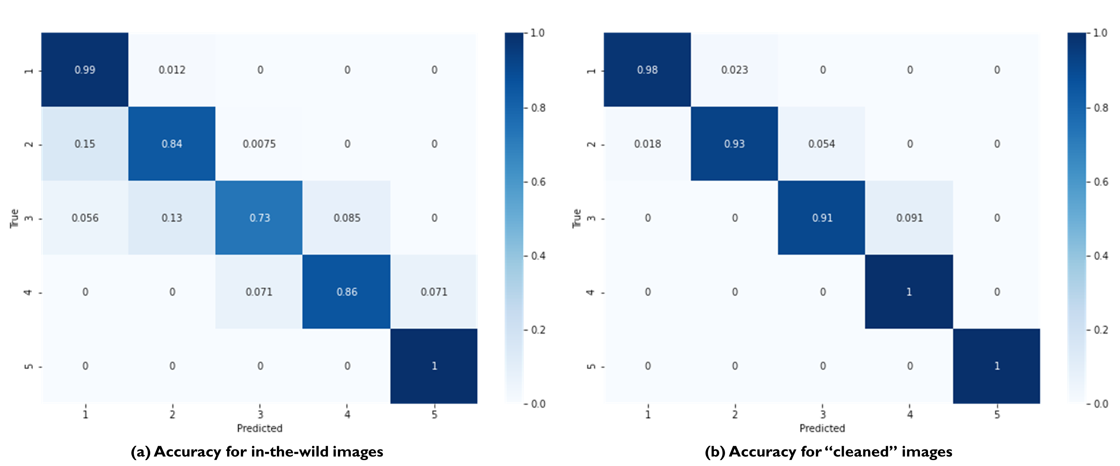
Fig. 3.2.2.6 Confusion matrices for the number of floors predictor used in this study.

Attribute: MeanRoofHt

The elevation of the bottom plane of the roof (lowest edge of roof line) and elevation of the roof (peak of gable or apex of hip) are estimated with respect to grade (in feet) from street-level imagery. These geometric properties are defined visually for common residential coastal typologies in Fig. 3.2.2.7. The mean height of the roof system is then derived as the average of these dimensions.

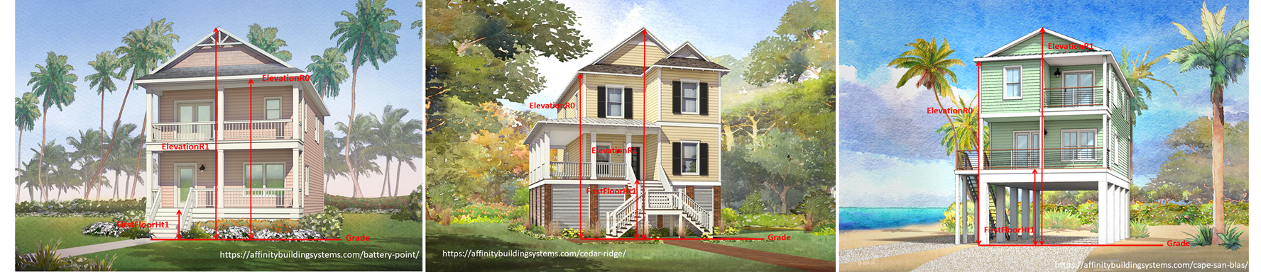
Fig. 3.2.2.7 Schematics demonstrating elevation quantities for different foundation systems common in coastal areas.

The MeanRoofHt is based on the following AI technique. Fig. 2.2.2.4 plots the predicted roof height versus the number of floors of the inventory.

As in any single-image metrology application, extracting the building elevations from imagery requires:

1. Rectification of image perspective distortions, typically introduced during capturing of an image capture.

2. Determining the pixel counts representing the distances between ends of the objects or surfaces of interest (e.g., for first-floor height, the orthogonal distance between the ground and first-floor levels).

3. Converting these pixel counts to real-world dimensions by matching a reference measurement with the corresponding pixel count.

Given that the number of street-level images available for a building can be limited and sparsely spaced, a single image rectification approach was deemed most applicable for regional-scale inventory development. The first step in image rectification requires detecting line segments on the front face of the building. This is performed by using the L-CNN end-to-end wireframe parsing method. Once the segments are detected, vertical and horizontal lines on the front face of the building are automatically detected using RANSAC line fitting based on the assumptions that line segments on this face are the predominant source of line segments in the image and the orientation of these line segments change linearly with their horizontal or vertical position depending on their predominant orientation. The Another support vector model implemented for image rectification focuses on the street-facing plane of the building in an image, and, based on the Manhattan World assumption, (i.e., all surfaces in the world are aligned with two horizontal and one vertical dominant directions) iteratively transforms the image such that horizontal edges on the facade plain lie parallel to each other, and its vertical edges are orthogonal to the horizontal edges.

In order to automate the process of obtaining the pixel counts for the ground elevations, a facade segmentation model was trained to automatically label ground, facade, door, window, and roof pixels in an image. The segmentation model was trained using DeepLabV3 architecture on a ResNet-101 backbone, pretrained on PASCAL VOC 2012 segmentation dataset, using a facade segmentation dataset of 30,000 images supplemented with relevant portions of ADE20K segmentation dataset. The peak model performance was attained using the Adam optimizer at a learning rate of 0.001 (batch size: 4), after 40 epochs. The conversion between pixel dimensions and real-world dimensions were attained by use of field of view and camera distance information collected for each street-level imagery.

Fig. 2.2.2.4 shows a scatter plot of the AI predicted mean roof heights vs AI-predicted number of floors. A general trend observed in this plot is that the roof height increases with the number of floors, which is in line with the general intuition.

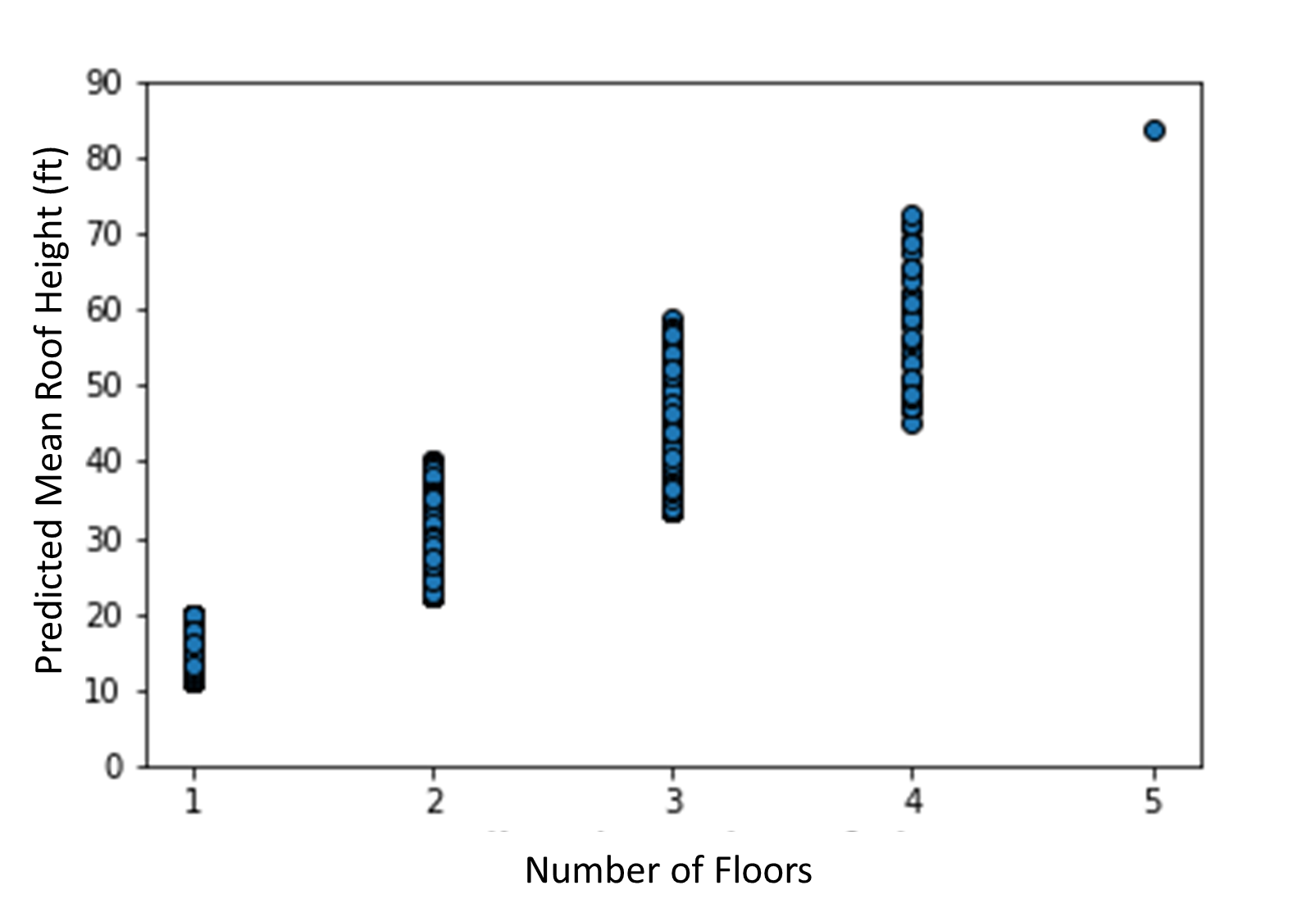
Fig. 3.2.2.8 AI-predicted MeanRoofHt versus number of floors.

Attribute: RoofSlope

RoofSlope is calculated as the ratio between the roof height and the roof run. Roof height is obtained by determining the difference between the bottom plane and apex elevations of the roof as defined in the Attribute: MeanRoofHt section. Roof run is determined as half the smaller dimension of the building, as determined from the dimensions of the building footprint. Fig. 3.2.2.9 displays the AI-predicted mean roof height versus the AI-precited roof pitch ratios. As expected, very little correlation between these two parameters are observed.

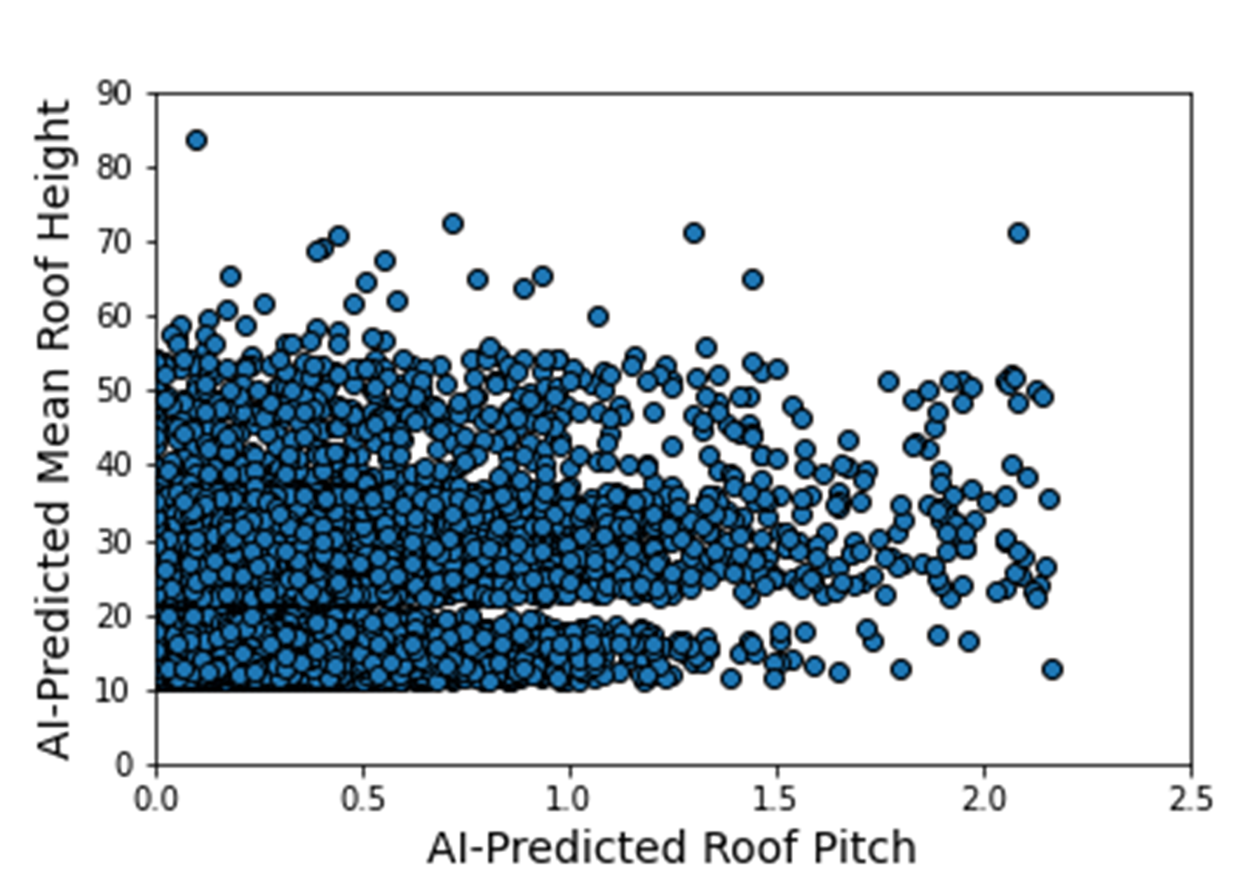
Fig. 3.2.2.9 AI-predicted RoofSlope versus mean roof height.

3.2.3. Phase III: Augmentation Using Third-Party Data, Site-specific Observations, and Existing Knowledge

The AI-generated building inventory is further augmented with multiple sources of information, including the third-party datasets, site-specific statistics summarized from observations, and existing knowledge and engineering judgement. The following attributes are obtained or derived from third-party data.

Attribute: DWS II

Design Wind Speed for Risk Category II construction in mph (ASCE 7-16), was obtained by queries to the ATC Hazards by Location API ([ATC20]).

Attribute: LULC

Land use code is downloaded from WebGIS. Each land use class is represented by a integer as listed in Table 3.2.1.1

Attribute: YearBuilt

We initially derived the year built information based on the National Structure Inventory (NSI), which contains year built information for geocoded addresses in the region of interest. It should be noted that not all buildings are included in the NSI dataset and the geocodes of the addresses do not match perfectly with building locations, as shown in Fig. 3.2.3.1.

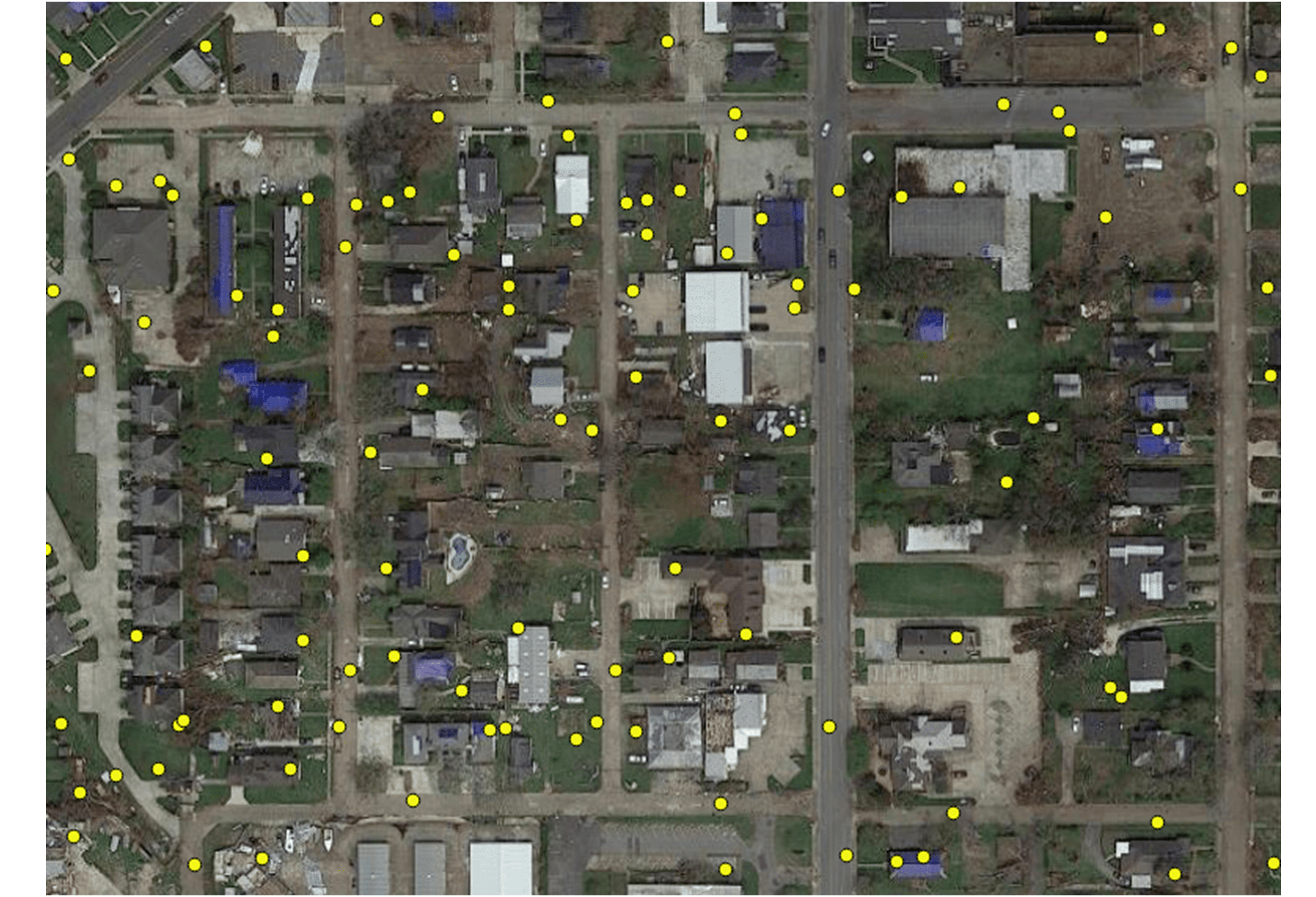
Fig. 3.2.3.1 National Structure Inventory data points.

To address this issue, SURF ([Wang19]) is employed to construct and train a neural network on the year built information from National Structure Inventory (NSI). The neural network is then used to predict the year built information for each building based on the spatial patterns it learned from the NSI dataset. The theory of using neural networks to learn the spatial patterns in data and to predict for missing values is detailed here. The result is shown in Fig. 3.2.3.2.

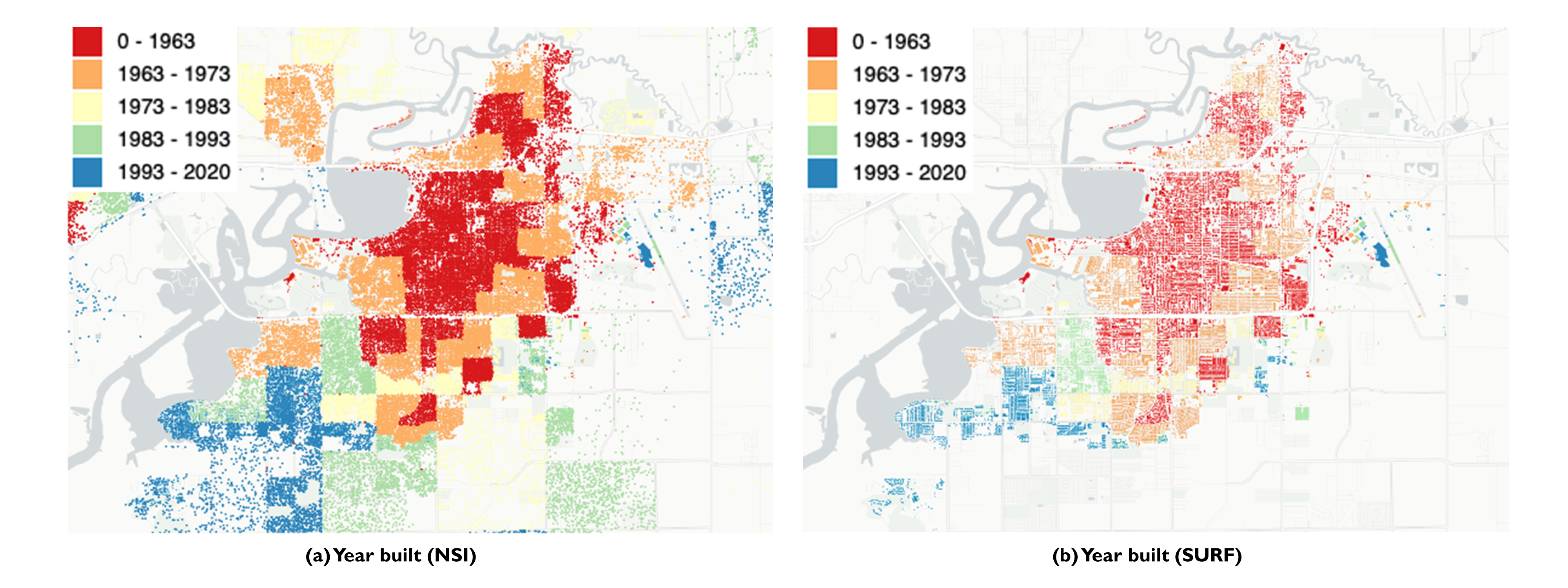
Fig. 3.2.3.2 Comparison of year built between NSI and SURF.

In parallel to this exploration, Zillow also provides the year built information for many of the residual buildings in the studied region.

Similar to the implementation of NSI dataset, the 1182 data points of year built from Zillow are used to train a neural network, Fig. 3.2.3.3 shows the verification of the trained neural network (predicted vs. true values, Zillow dataset). More than \(85%\) buildings have prediction errors less than 20 years.

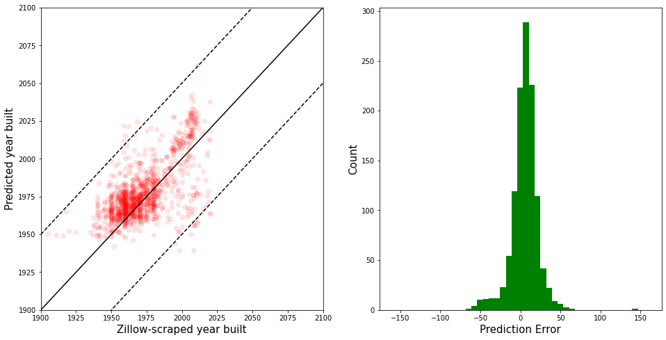
Fig. 3.2.3.3 SURF-predicted vs. original year built from Zillow dataset.

The neural network is used to predict the year built information for the entire Lake Charles inventory. Fig. 3.2.3.4 contrast the resulting SURF-Zillow and the SURF-NSI year built spatial distribution. The difference in year built is relatively small for the downtown buildings (~1960s) but increases at the bounds with a maximum of 80 years. The Zillow-trained classifier is undergoing continued improvements and will be released with the next version of this testbed. The current version of the testbed will thus use the NSI data as the basis for the Year Built Attribute

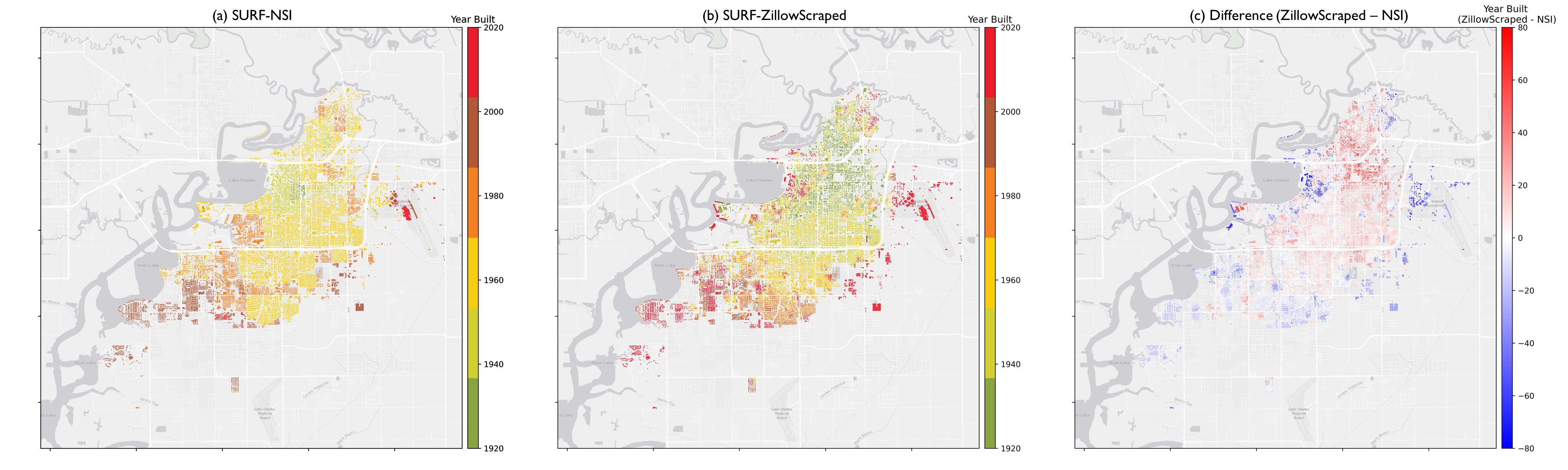
Fig. 3.2.3.4 SURF-NSI vs. SURF-Zillow: year built information.

Attribute: Garage

A garage detector utilizing EfficienDet object detection architecture was trained to identify the existence of attached garage and carport structures in street-level imagery of the buildings included in the Lake Charles inventory. Properties are either classified as having an attached garage or not having an attached garage (which includes both detached garages and homes with no garage) The model was trained on the EfficientDet-D4 architecture with dataset of 1,887 images, using 80% for training, 10% for validation, and 10% for testing of the model. Similar to the number of floors detector model, initial weights of this model were set to model weights of the (pretrained) object detection model that, at the time, achieved state-of-the-art performance on the 2017 COCO Detection set. For this task, the peak detector performance was attained using the Adam optimizer at a learning rate of 0.0001 (batch size: 2) after 25 epochs. Fig. 3.2.3.5 shows sample garage detections performed by the model.

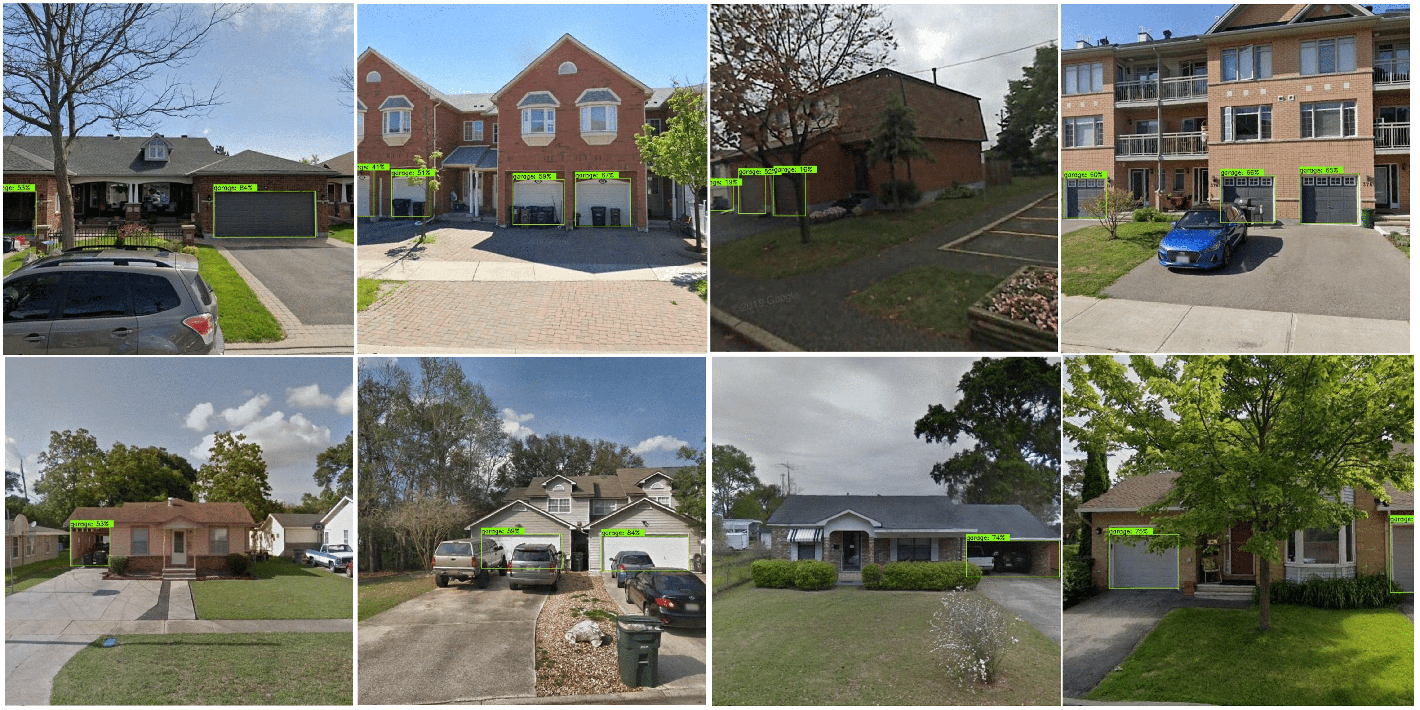
Fig. 3.2.3.5 Samples of the garage detection model showing successful identification of attached garages and carports.

On the test set, the model achieves an accuracy of 92%. Fig. 3.2.3.6 shows the confusion matrix of the model classifications on the test set. On a seperate test set consisting of images from only Lake Charles, model performance is lower at 71%. Fig. 3.2.3.6 (b) shows the confusion matrix for model predictions on this latter dataset.

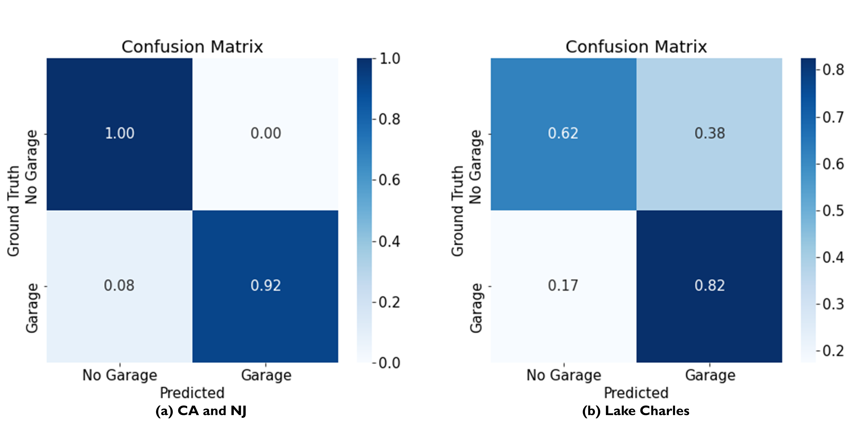
Fig. 3.2.3.6 Confusion matrices for the garage predictor used in this study. The matrix on the left (a) shows the model’s prediction accuracy when tested on a set of 189 images randomly selected from CA and NJ. The matrix on the right (b) depicts the model accuracy on images selected from the Lake Charles area.

Attribute: BuildingType

Based on information found in the National Structure Inventory, 89% of residential buildings (single-family and multi-family) are wood, the rest are masonry. In the analysis, we conservatively assume all residential buildings are wood.

Attribute: AvgJanTemp

The average temperature in Lake Charles in January is above the critical value of 25F, based on NOAA average daily temperature. Referring Table 3.2.1.1, we used “Above” for the buildings in the studied inventory.

3.2.4. Populated Inventories

Executing this three-phase process resulted in the assignment of all required attributes at the asset description stage of the workflow for the Lake Charles building inventory, and Table 3.2.4.1 shows example data samples. The entire inventory can be accessed here.

Table 3.2.4.1 Illustrative sample of building in Lake Charles Inventory.

BldgID	RoofShape	PlanArea	Longitude	Latitude	LULC	DWSII	BuildingType	OccupancyClass	AvgJanTemp	Garage	NumberOfStories	MeanRoofHt	RoofSlope	YearBuilt
1	Hip	745	-93.19	30.27	43	128.7	Wood	RES3	Above	0	1	15	0.25	1962
2	Gable	250	-93.19	30.26	11	129	Wood	RES1	Above	0	1	12.97	0.21	1970
3	Gable	170	-93.19	30.26	11	129	Wood	RES1	Above	0	1	16.28	0.22	1969
4	Gable	142	-93.18	30.26	11	129	Wood	RES1	Above	1	2	34.58	0.12	1974
5	Gable	270	-93.18	30.26	11	128.9	Wood	RES1	Above	1	1	14.22	0.33	1968
6	Gable	160	-93.18	30.27	11	128.8	Wood	RES1	Above	1	1	16.06	0.3	1957
7	Hip	257	-93.21	30.22	11	130.2	Wood	RES1	Above	0	1	16.18	0.16	1950
8	Hip	143	-93.21	30.22	11	130.2	Wood	RES1	Above	0	2	22.68	0.11	1944
9	Hip	290	-93.21	30.23	11	130.1	Wood	RES1	Above	0	2	28.98	0.33	1941
10	Gable	229	-93.21	30.23	12	130	Wood	RES3	Above	0	2	30.38	0.45	1941
11	Gable	213	-93.20	30.25	11	129.3	Wood	RES3	Above	1	1	13.48	0.65	1959
12	Gable	125	-93.19	30.25	11	129.3	Wood	RES1	Above	0	1	17.19	0.17	1955
13	Gable	128	-93.19	30.25	11	129.3	Wood	RES1	Above	1	2	31.5	0.92	1956
14	Gable	202	-93.19	30.25	11	129.3	Wood	RES1	Above	0	1	15.95	0.69	1959
15	Flat	98	-93.19	30.25	11	129.3	Wood	RES1	Above	0	1	16.93	0.65	1955
16	Hip	193	-93.20	30.25	11	129.3	Wood	RES1	Above	1	2	30.1	1.28	1958
17	Hip	303	-93.19	30.25	11	129.2	Wood	RES3	Above	0	1	15	0.25	1959
18	Hip	288	-93.20	30.24	13	129.6	Wood	RES1	Above	1	1	13.06	0.45	1964
19	Flat	108	-93.20	30.24	11	129.5	Wood	RES1	Above	1	1	12.8	0.06	1965
20	Gable	204	-93.20	30.25	11	129.4	Wood	RES1	Above	1	3	36.12	0.65	1958

ATC20

ATC (2020b), ATC Hazards By Location, https://hazards.atcouncil.org/, Applied Technology Council, Redwood City, CA.

Wang19

Wang C. (2019), NHERI-SimCenter/SURF: v0.2.0 (Version v0.2.0). Zenodo. http://doi.org/10.5281/zenodo.3463676

Microsoft18

Microsoft (2018), US Building Footprints. https://github.com/Microsoft/USBuildingFootprints

FEMA21

FEMA (2021), Hazus Inventory Technical Manual. Hazus 4.2 Service Pack 3. Federal Emergency Management Agency, Washington D.C.