3.8. Getting Started

3.8.1. Running Testbed

R2D Interface

One approach to run the testbed simulation is via the R2D application. After successfully downloading and launching, the major steps for setting up the run are listed as follows:

1. Set the Units in the GI panel as shown in Fig. 2.8.1.2 and check interested output files.

   

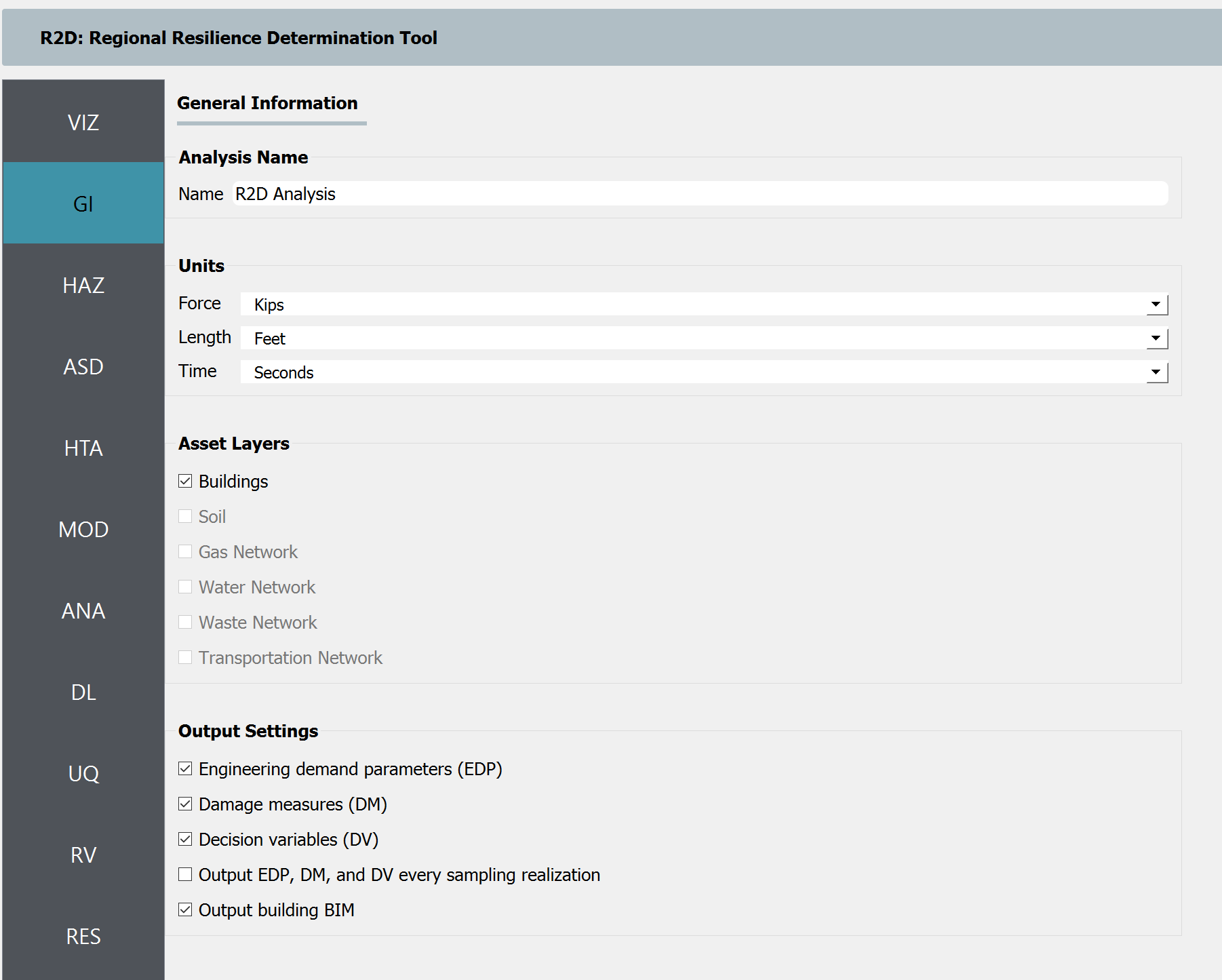
   Fig. 3.8.1.1 R2D GI setup.

2. Download and unzip the HurricaneLaura_MappedPWS. Set the Event File Listing Wind Field in the HAZ panel to the “EventGrid.csv” in the unzipped “IMs” folder. The app would automatically load the directory (Fig. 2.8.1.3). And the Units of Event Input File should be “Miles per hour”.

   

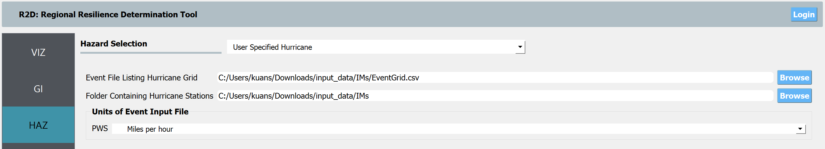
   Fig. 3.8.1.2 R2D HAZ setup.

3. Download the BIM_LakeCharles_Full.csv (under 01. Input: BIM - Building Inventory Data folder). Select CSV to BIM in the ASD panel and set the Import Path to “BIM_LakeCharles_Full.csv” (Fig. 2.8.1.4). Specify the building IDs that you would like to include in the simulation (e.g., 1-26516 for the entire inventory - note this may take very long time to run on a local machine, so it is suggested to first test with a small sample like 1-100 locally and then submit the entire run to DesignSafe - see more details in Fig. 2.8.1.11).

   

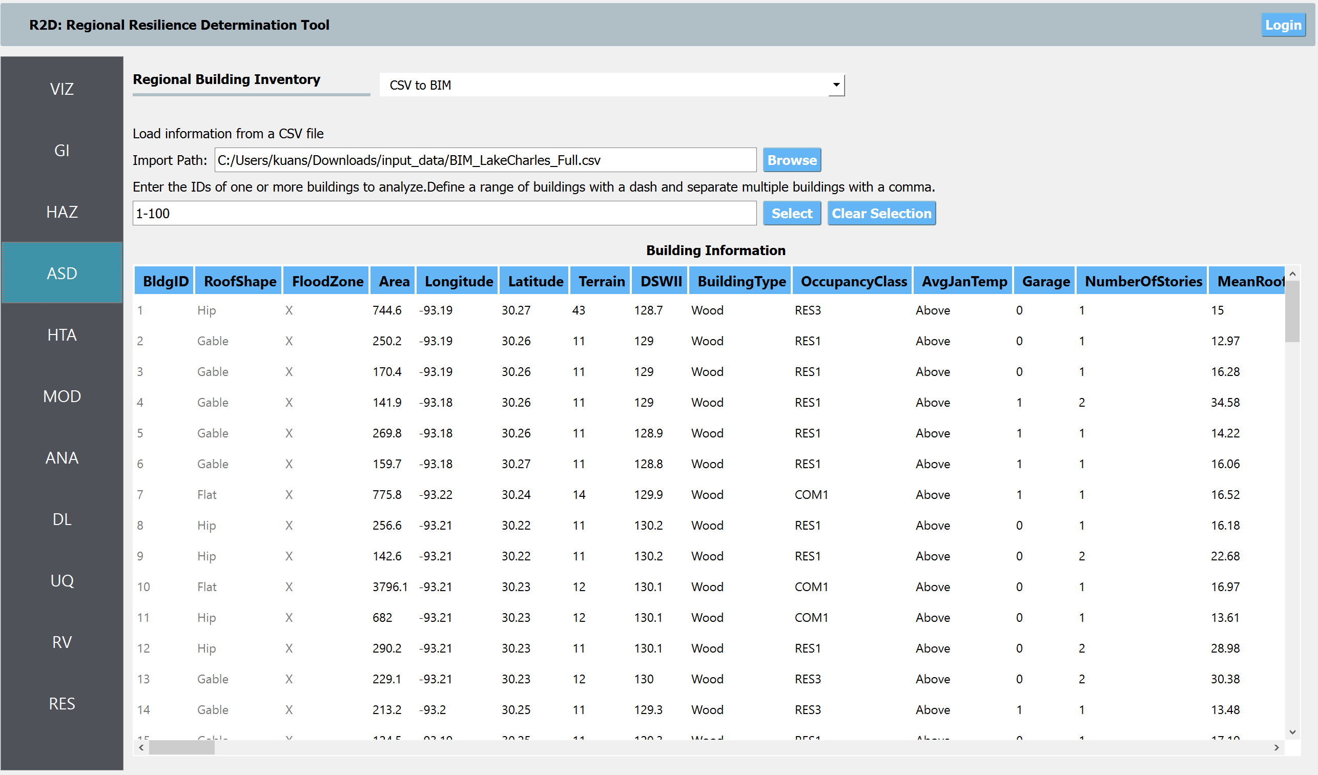
   Fig. 3.8.1.3 R2D ASD setup.

4. Set the Regional Mapping and SimCenterEvent in the HTA panel (e.g., Fig. 2.8.1.5).

   

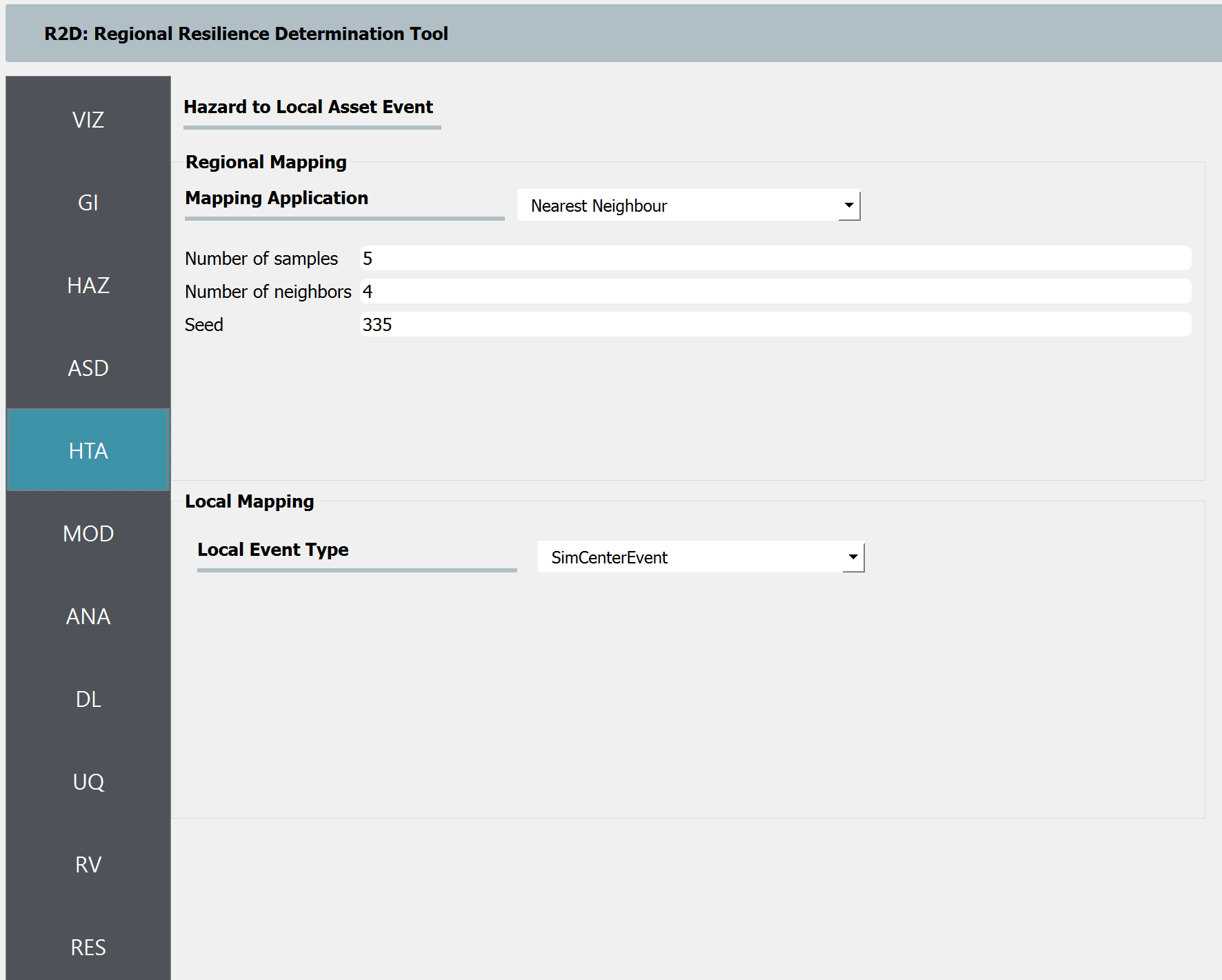
   Fig. 3.8.1.4 R2D HTA setup.

5. Set the “Building Modeling” in MOD panel to “None”.

   

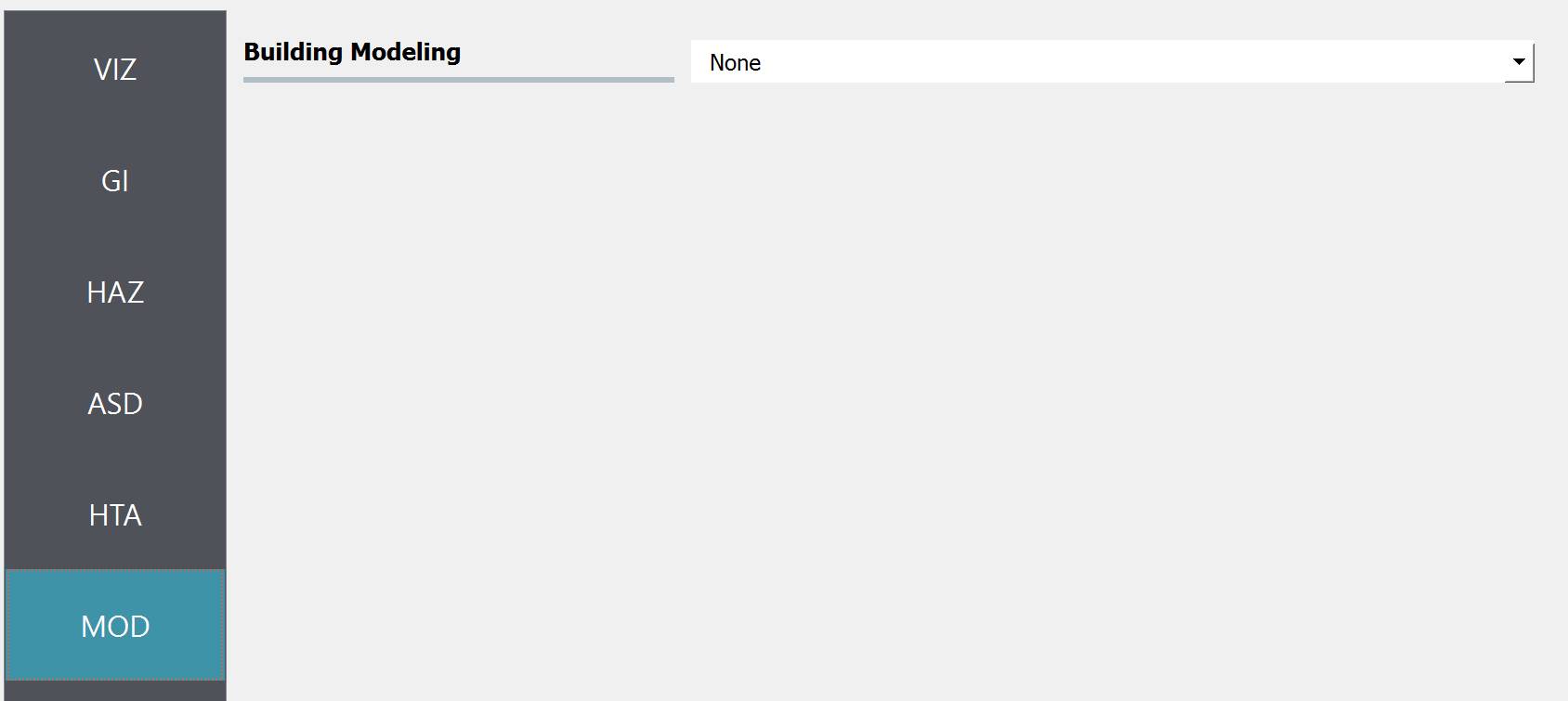
   Fig. 3.8.1.5 R2D MOD setup.

6. Set the “Building Analysis Engine” in ANA panel to “IMasEDP”.

   

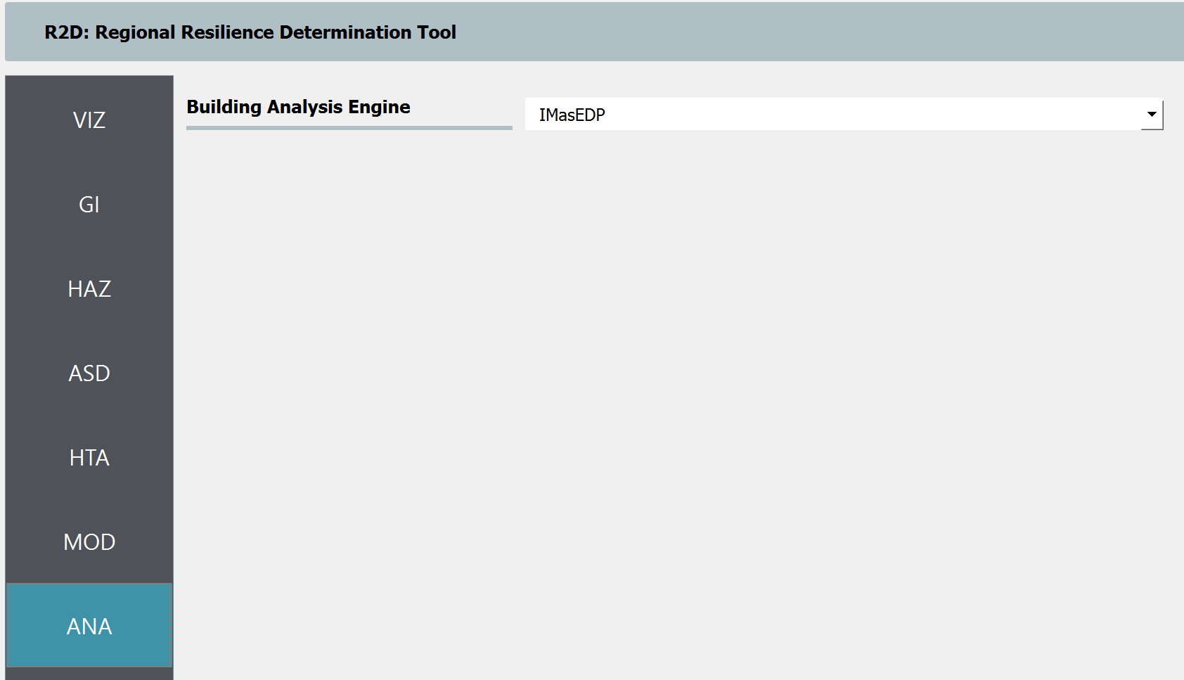
   Fig. 3.8.1.6 R2D ANA setup.

7. Set the “Damage and Loss Method” in DL panel to “HAZUS MH HU”. Download the rulset scripts from DesignSafe PRJ-3207 (under 03. Input: DL - Rulesets for Asset Representation/scripts folder) and set the Auto populate script to “auto_HU_LA.py” (Fig. 2.8.1.8). Note please place the rulset scripts in an individual folder so that the application could copy and load them later.

   

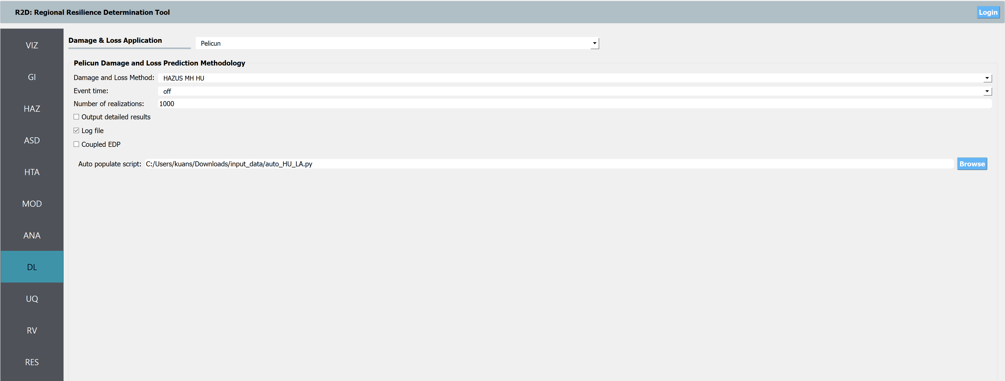
   Fig. 3.8.1.7 R2D DL setup.

8. Set the “UQ Application” in UQ panel to “None”.

   

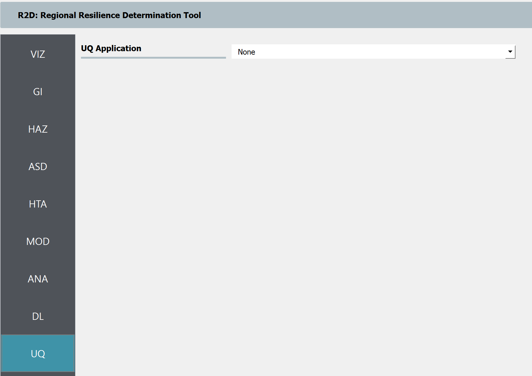
   Fig. 3.8.1.8 R2D UQ setup.

After setting up the simulation, please click the RUN to execute the analysis. Once the simulation completed, the app would direct you to the RES panel (Fig. 2.8.1.10) where you could examine and export the results.

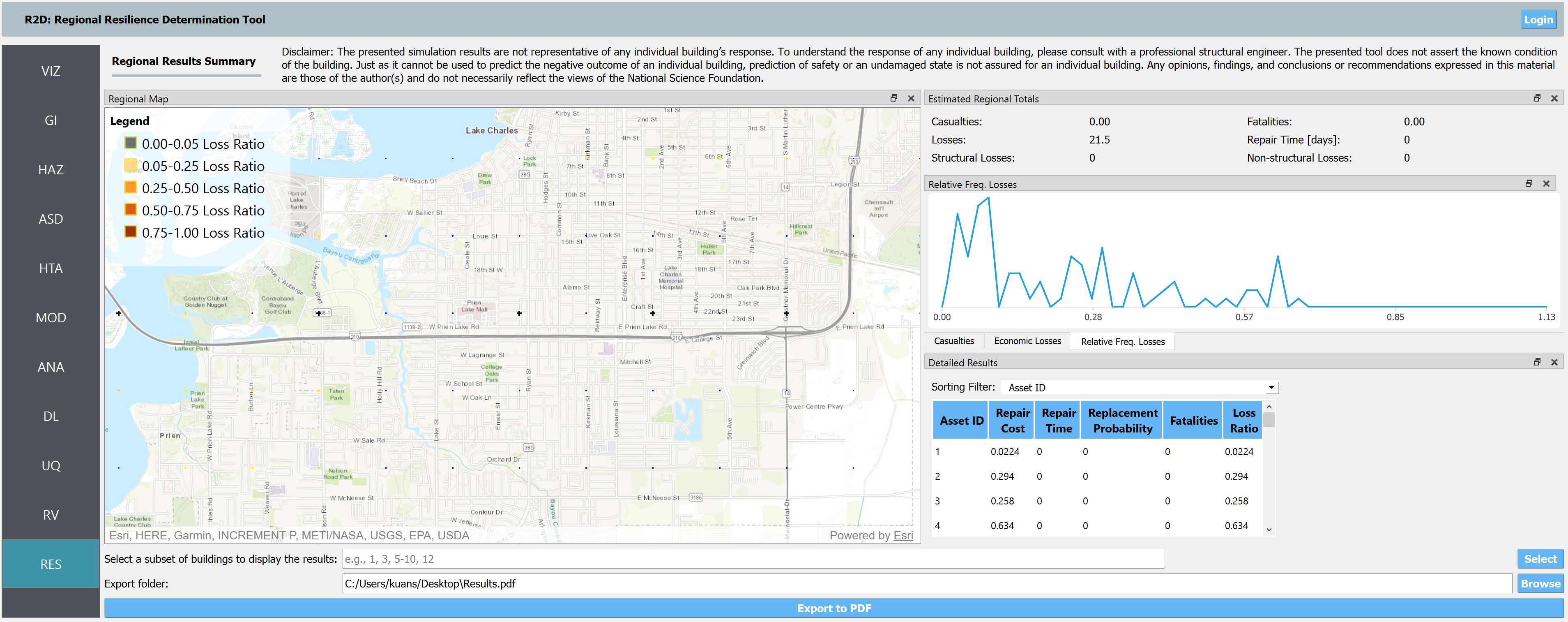
Fig. 3.8.1.9 R2D RES panel.

For simulating the damage and loss for a large region of interest (please remember to reset the building IDs in ASD), it would be efficient to submit and run the job to DesignSafe on Stampede2. This can be done in R2D by clicking RUN at DesignSafe (one would need to have a valid DesignSafe account for login and access the computing resource). Fig. 2.8.1.11 provides an example configuration to run the analysis (and please see R2D User Guide for detailed descriptions). The individual building simulations are paralleled when being conducted on Stampede2 which accelerate the process. It is suggested for the entire building inventory in this testbed to use 15 minutes with 96 Skylake (SKX) cores (e.g., 2 nodes with 48 processors per node) to complete the simulation. One would receive a job failure message if the specified CPU hours are not sufficient to complete the run. Note that the product of node number, processor number per node, and buildings per task should be greater than the total number of buildings in the inventory to be analyzed.

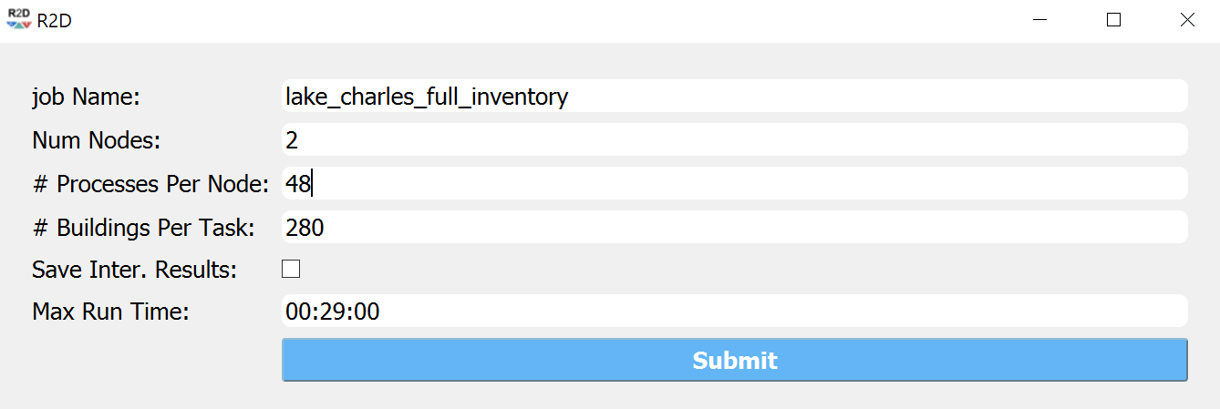
Fig. 3.8.1.10 R2D - Run at DesignSafe (configuration).

Users could monitor the job status and retrieve result data by GET from DesignSafe button (Fig. 2.8.1.12). The retrieved data include four major result files, i.e., BIM.hdf, EDP.hdf, DM.hdf, and DV.hdf. R2D also automatically converts the hdf files to csv files that are easier to work with. While R2D provides basic visualization functionalities (Fig. 2.8.1.10), users could access the data which are downloaded under the remote work directory, e.g., /Documents/R2D/RemoteWorkDir (this directory is machine specific and can be found in File->Preferences->Remote Jobs Directory). Once having these result files, users could extract and process interested information - the next section will use the results from this testbed as an example to discuss more details.

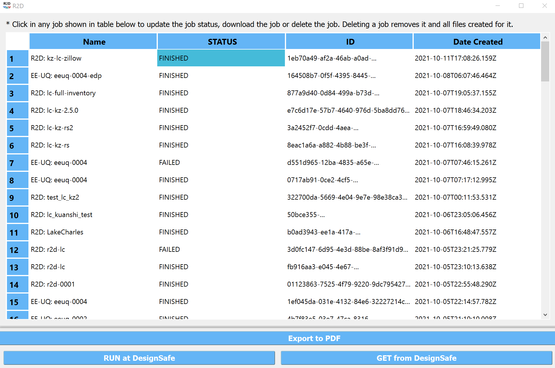
Fig. 3.8.1.11 R2D GET from DesignSafe.

3.8.2. Regional Results (NSI-Based Year Built)

The specific entries included in the BIM.hdf file are explained in Asset Description and specifically Table 3.2.1.1. It is important to note that this BIM.hdf file is an enhanced version of the input BIM file, including additional information necessary for the loss estimation (fields added through rulesets explained in Asset Representation). Additionally, the BIM.hdf file includes only the buildings in the original inventory file that could be successfully executed by the workflow, e.g., satisfied conditions in the rulesets necessary to assign requisite attributes. If there are errors in the assignment process, the output BIM.hdf file will have fewer buildings than the original input BIM file. As such, this expanded inventory file output by R2D should be used for subsequent analyses, rather than the original inventory used to run the simulation in Step 3 above. The EDP.hdf summarizes the EDP realizations. The DM.hdf and DV.hdf files summarizes the statistics of damage states and estimated loss metrics. These results of this testbed can be accessed in the DesignSafe project, along with the Jupyter notebook used to visualize them. The zip file consists of (1) four result hdf files (BIM.hdf, EDP.hdf, DM.hdf, and DV.hdf), (2) four parsed result files (in .csv), (3) Input inventory csv file, (4) two jupyter notebook scripts, and (5) a requirement txt file listing the dependencies. post-process.ipynb can be run locally and first-time users are suggested to run the first cell to install necessary packages, and post-processing_designsafe.ipynb can be run on DesignSafe Jupyter Notebook if one uploads the entire folder to the Data Depot. Note users are suggested to find more detailed descriptions about the data attributes in the DV.csv in the pelicun documentation.

Fig. 3.8.2.1 (a) and (b) show the sample figures for the geospatial distribution of populated terrain type and second water resistance of the building inventory. The influence of different building attributes on the damage and loss results will be investigated in Validation Results The geospatial distribution of estimated wind damage states and losses under Hurricane Laura are shown in Fig. 3.8.2.2 (a) and (b), respectively. Referring to Fig. 3.8.2.2 (c), most of the buildings in the studied region (75%) have relatively low to moderate damage (expected Damage State less than 2.0) due to the wind hazard. Referring to Fig. 3.8.2.2 (c), about 5% buildings would expected damage states lower than DS-1 and only about 5% buildings would expect to have damage states exceeding DS-3. The CDF of resulting loss ratios is shown in Fig. 3.8.2.2 (d) where about 20% buildings would expect a loss less than 10% of the total reconstruction cost, and about 30% buildings could see a loss more than 35% of the total reconstruction cost.

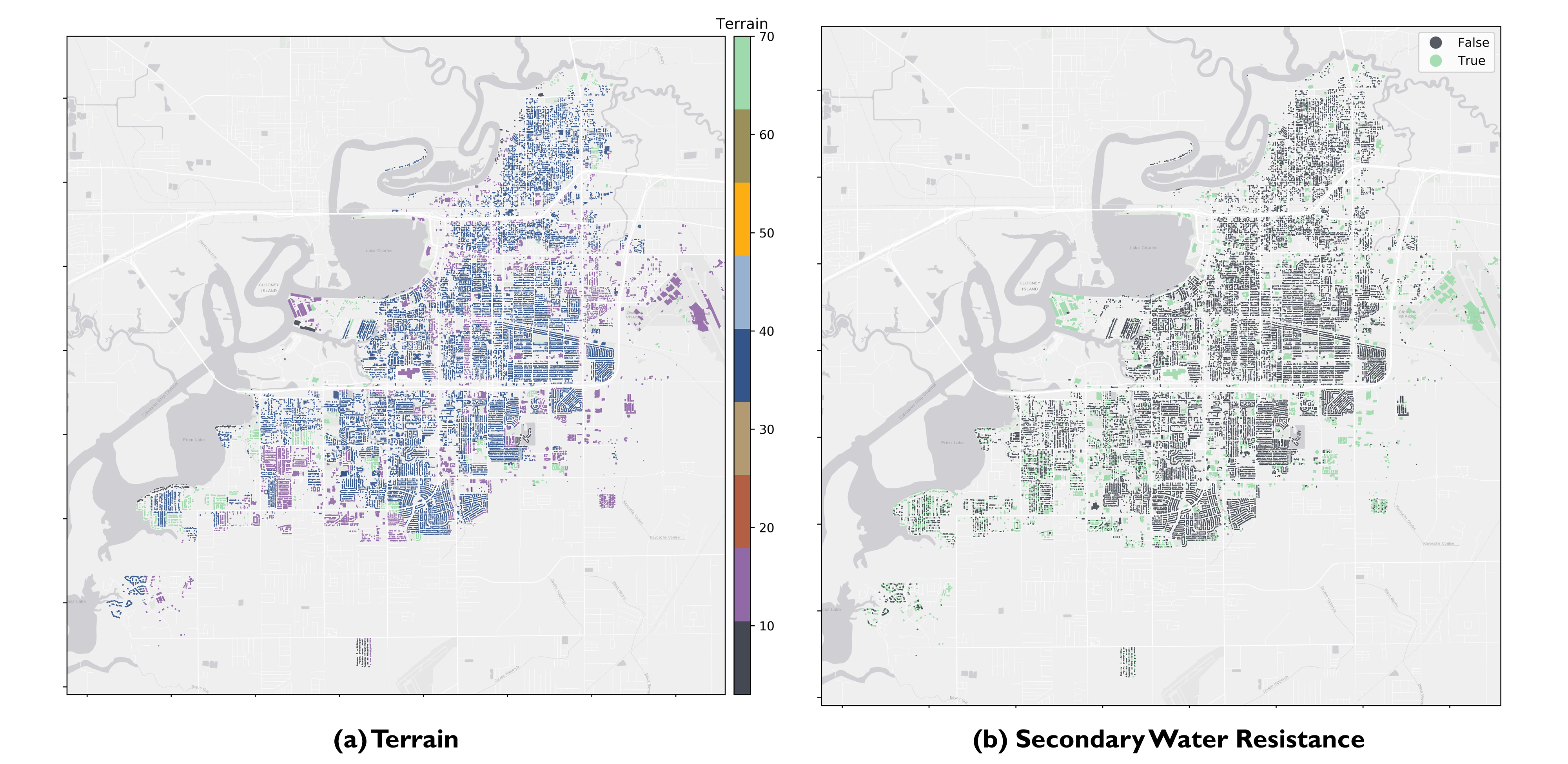
Fig. 3.8.2.1 Terrain and second water resistance features populated and used in the simulation.

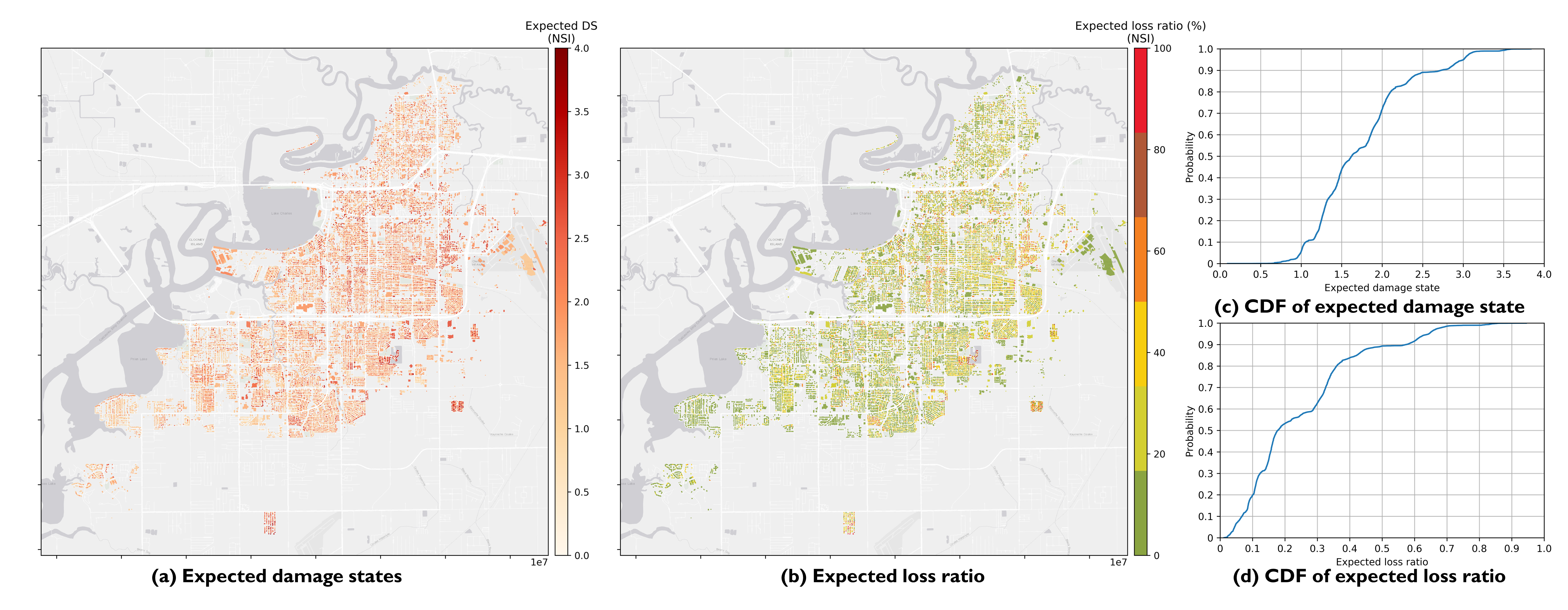
Fig. 3.8.2.2 Estimated regional damage states and loss ratios.