2.9.1.1. Forward Propagation Methods

The forward propagation analysis provides probabilistic understanding of output variables by producing sample realizations and statistical moments (mean, standard deviation, skewness, and kurtosis) of the quantities of interest. Currently four sampling methods are available:

1. Monte Carlo Sampling (MCS)

2. Latin Hypercube Sampling (LHS)

and sampling based on surrogate models, including:

3. Gaussian Process Regression (GPR)

4. Polynomial Chaos Expansion (PCE)

Depending on the option selected, the user must specify the appropriate input parameters. For instance, for MCS, the number of samples specifies the number of simulations to be performed, and providing a seed value for the pseudo-random number generator allows the user to reproduce the sampling results multiple times. The user selects the sampling method from the dropdown Dakota Method Category menu. Additional information regarding sampling techniques offered in Dakota can be found here.

Monte Carlo Sampling (MCS)

MCS is among the most robust and universally applicable sampling methods. Moreover, the convergence rate of MCS methods are independent of the problem dimensionality, albeit the convergence rate of such MCS methods is relatively slow at \(N^{-1/2}\). In MCS, a sample drawn at any step is independent of all previous samples.

figMCS shows the input panel corresponding to the Monte Carlo Sampling setting. Two input parameters need to be specified: (1) the number of samples of the output to be produced, which is equal to the number of times the model is evaluated, and (2) the seed for the pseudo-random number generator.

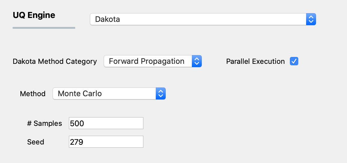
Fig. 2.9.1.1.1 Monte Carlo Sampling input panel.

Latin Hypercube Sampling (LHS)

Latin hypercube sampling (LHS) is a type of stratified sampling approach. To achieve a better convergence, LHS evenly spreads out the samples to cover the whole range of the input domain. Each sample from LHS effectively represents each of N equal probability intervals of a cumulative density function.

figLHS shows the input panel corresponding to the Latin hypercube sampling (LHS) scheme. Two input parameters need to be specified: (1) the number of samples of the output to be produced, which is equal to the number of times the model is evaluated, and (2) the seed for the pseudo-random number generator.

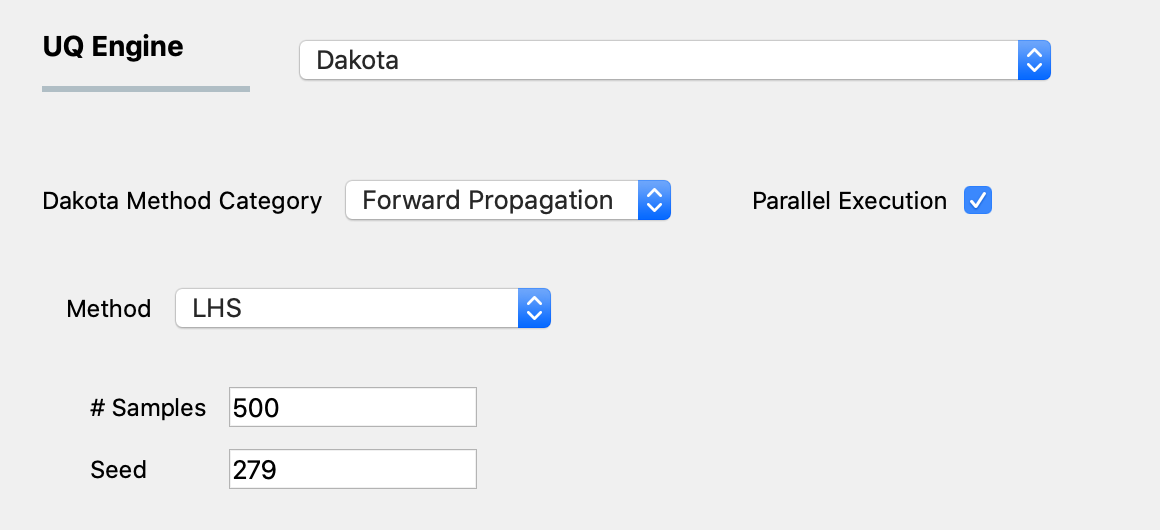
Fig. 2.9.1.1.2 Latin Hypercube Sampling input panel.

Gaussian Process Regression (GPR)

For the problems in which computationally expensive models are involved, conventional sampling schemes such as LHS and MCS can be extremely time-consuming. In such case, a surrogate model can be constructed based on a smaller number of simulation runs, and then the surrogate model can be used to efficiently generate the required number of samples replacing the expensive simulations.

Gaussian Process Regression (GPR), also known as Kriging is one of the well-established surrogate techniques, which constructs an approximated response surface based on Gaussian process modeling and covariance matrix optimizations. figGPR shows the input panel for the GPR model that consists of training and sampling panels.

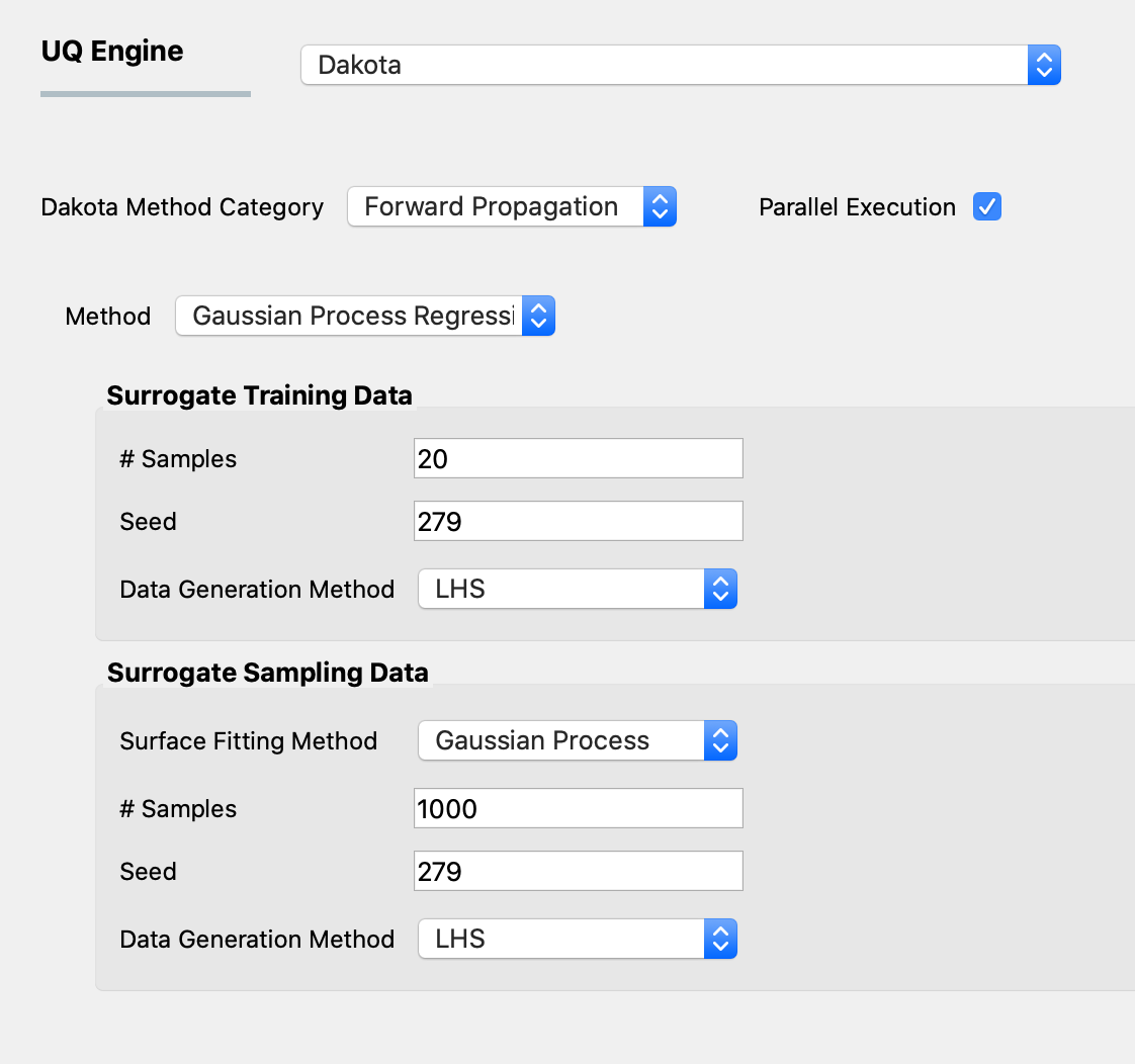
Fig. 2.9.1.1.3 GPR forward propagation input panel.

In the Surrogate Training Data panel, the users specify the number of samples of the output of the computationally expensive model to be select either Monte Carlo Sampling or Latin Hypercube Sampling to generate sample output values from the computationally expensive model, which, along with the corresponding input values are used to train the surrogate models.

Other surrogate models, different from Gaussian process regression are also available in the drop-down menu titled Surface Fitting Method. All thse surrogate models utilize either Monte Carlo Sampling or Latin Hypercube Sampling to generate sample output values, which, along with the corresponding input values are used to train the surrogate models.

Polynomial Chaos Expansion (PCE)

Response surface can be approximated using Polynomial Chaos Expansion (PCE) model as well. Similar to the input GPR panel, input panel for PCE model shown in figPCE consists of training and sampling parts. The input parameters in the surrogate training data set specify the dataset used for training the surrogate model, while the parameters in the surrogate sampling data are related to the samples generated using the surrogate. Extreme care must be taken in specifying the parameters of the training dataset to results in an accurate response surface approximation.

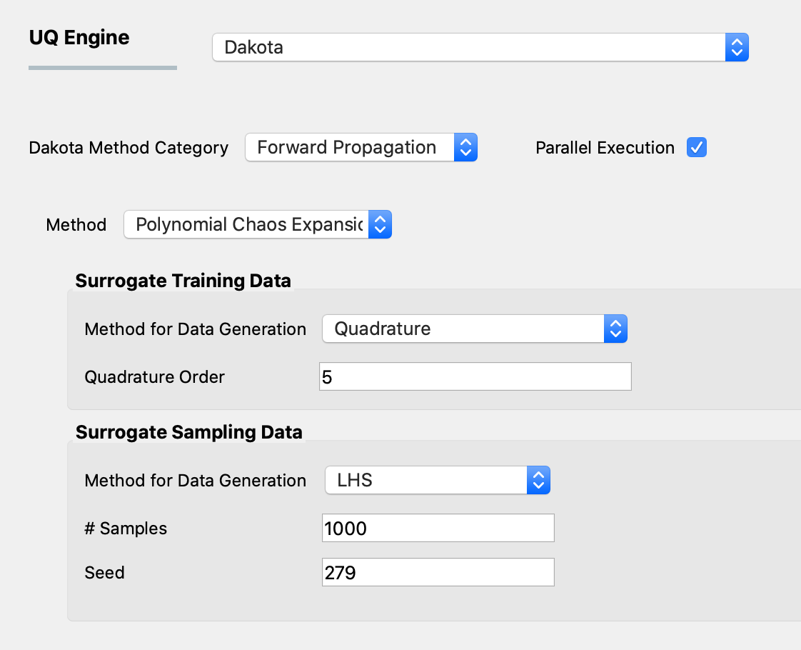
Fig. 2.9.1.1.4 PCE forward propagation input panel.

If the user is not familiar with the training parameters of the surrogates, it is recommended to refrain from using the surrogates (PCE in particular) and instead use conventional sampling such as MCS and LHS, even at a higher computational cost.